Векторная модель исправления ошибок - Решение и исправление самых разных ошибок на TopOshibok.ru

From Wikipedia, the free encyclopedia

An error correction model (ECM) belongs to a category of multiple time series models most commonly used for data where the underlying variables have a long-run common stochastic trend, also known as cointegration. ECMs are a theoretically-driven approach useful for estimating both short-term and long-term effects of one time series on another. The term error-correction relates to the fact that last-period’s deviation from a long-run equilibrium, the error, influences its short-run dynamics. Thus ECMs directly estimate the speed at which a dependent variable returns to equilibrium after a change in other variables.

History[edit]

Yule (1926) and Granger and Newbold (1974) were the first to draw attention to the problem of spurious correlation and find solutions on how to address it in time series analysis.^[1]^[2] Given two completely unrelated but integrated (non-stationary) time series, the regression analysis of one on the other will tend to produce an apparently statistically significant relationship and thus a researcher might falsely believe to have found evidence of a true relationship between these variables. Ordinary least squares will no longer be consistent and commonly used test-statistics will be non-valid. In particular, Monte Carlo simulations show that one will get a very high R squared, very high individual t-statistic and a low Durbin–Watson statistic. Technically speaking, Phillips (1986) proved that parameter estimates will not converge in probability, the intercept will diverge and the slope will have a non-degenerate distribution as the sample size increases.^[3] However, there might be a common stochastic trend to both series that a researcher is genuinely interested in because it reflects a long-run relationship between these variables.

Because of the stochastic nature of the trend it is not possible to break up integrated series into a deterministic (predictable) trend and a stationary series containing deviations from trend. Even in deterministically detrended random walks spurious correlations will eventually emerge. Thus detrending does not solve the estimation problem.

In order to still use the Box–Jenkins approach, one could difference the series and then estimate models such as ARIMA, given that many commonly used time series (e.g. in economics) appear to be stationary in first differences. Forecasts from such a model will still reflect cycles and seasonality that are present in the data. However, any information about long-run adjustments that the data in levels may contain is omitted and longer term forecasts will be unreliable.

This led Sargan (1964) to develop the ECM methodology, which retains the level information.^[4]^[5]

Estimation[edit]

Several methods are known in the literature for estimating a refined dynamic model as described above. Among these are the Engle and Granger 2-step approach, estimating their ECM in one step and the vector-based VECM using Johansen’s method.^[6]

Engle and Granger 2-step approach[edit]

The first step of this method is to pretest the individual time series one uses in order to confirm that they are non-stationary in the first place. This can be done by standard unit root DF testing and ADF test (to resolve the problem of serially correlated errors).
Take the case of two different series $x_{t}$ and $y_{t}$ . If both are I(0), standard regression analysis will be valid. If they are integrated of a different order, e.g. one being I(1) and the other being I(0), one has to transform the model.

If they are both integrated to the same order (commonly I(1)), we can estimate an ECM model of the form

$A(L)\,\Delta y_{t}=\gamma +B(L)\,\Delta x_{t}+\alpha (y_{t-1}-\beta _{0}-\beta _{1}x_{t-1})+\nu _{t}.$

If both variables are integrated and this ECM exists, they are cointegrated by the Engle–Granger representation theorem.

The second step is then to estimate the model using ordinary least squares: $y_{t}=\beta _{0}+\beta _{1}x_{t}+\varepsilon _{t}$
If the regression is not spurious as determined by test criteria described above, Ordinary least squares will not only be valid, but also consistent (Stock, 1987).
Then the predicted residuals ${\hat {\varepsilon _{t}}}=y_{t}-\beta _{0}-\beta _{1}x_{t}$ from this regression are saved and used in a regression of differenced variables plus a lagged error term

$A(L)\,\Delta y_{t}=\gamma +B(L)\,\Delta x_{t}+\alpha {\hat {\varepsilon }}_{t-1}+\nu _{t}.$

One can then test for cointegration using a standard t-statistic on $\alpha$ .
While this approach is easy to apply, there are numerous problems:

VECM[edit]

The Engle–Granger approach as described above suffers from a number of weaknesses. Namely it is restricted to only a single equation with one variable designated as the dependent variable, explained by another variable that is assumed to be weakly exogeneous for the parameters of interest. It also relies on pretesting the time series to find out whether variables are I(0) or I(1). These weaknesses can be addressed through the use of Johansen’s procedure. Its advantages include that pretesting is not necessary, there can be numerous cointegrating relationships, all variables are treated as endogenous and tests relating to the long-run parameters are possible. The resulting model is known as a vector error correction model (VECM), as it adds error correction features to a multi-factor model known as vector autoregression (VAR). The procedure is done as follows:

Step 1: estimate an unrestricted VAR involving potentially non-stationary variables
Step 2: Test for cointegration using Johansen test
Step 3: Form and analyse the VECM.

An example of ECM[edit]

The idea of cointegration may be demonstrated in a simple macroeconomic setting. Suppose, consumption $C_{t}$ and disposable income $Y_{t}$ are macroeconomic time series that are related in the long run (see Permanent income hypothesis). Specifically, let average propensity to consume be 90%, that is, in the long run $C_{t}=0.9Y_{t}$ . From the econometrician’s point of view, this long run relationship (aka cointegration) exists if errors from the regression $C_{t}=\beta Y_{t}+\varepsilon _{t}$ are a stationary series, although $Y_{t}$ and $C_{t}$ are non-stationary. Suppose also that if $Y_{t}$ suddenly changes by $\Delta Y_{t}$ , then $C_{t}$ changes by $\Delta C_{t}=0.5\,\Delta Y_{t}$ , that is, marginal propensity to consume equals 50%. Our final assumption is that the gap between current and equilibrium consumption decreases each period by 20%.

In this setting a change $\Delta C_{t}=C_{t}-C_{{t-1}}$ in consumption level can be modelled as $\Delta C_{t}=0.5\,\Delta Y_{t}-0.2(C_{t-1}-0.9Y_{t-1})+\varepsilon _{t}$ . The first term in the RHS describes short-run impact of change in $Y_{t}$ on $C_{t}$ , the second term explains long-run gravitation towards the equilibrium relationship between the variables, and the third term reflects random shocks that the system receives (e.g. shocks of consumer confidence that affect consumption). To see how the model works, consider two kinds of shocks: permanent and transitory (temporary). For simplicity, let $\varepsilon _{t}$ be zero for all t. Suppose in period t − 1 the system is in equilibrium, i.e. $C_{{t-1}}=0.9Y_{{t-1}}$ . Suppose that in the period t, disposable income $Y_{t}$ increases by 10 and then returns to its previous level. Then $C_{t}$ first (in period t) increases by 5 (half of 10), but after the second period $C_{t}$ begins to decrease and converges to its initial level. In contrast, if the shock to $Y_{t}$ is permanent, then $C_{t}$ slowly converges to a value that exceeds the initial $C_{{t-1}}$ by 9.

This structure is common to all ECM models. In practice, econometricians often first estimate the cointegration relationship (equation in levels), and then insert it into the main model (equation in differences).

References[edit]

^ Yule, Georges Udny (1926). «Why do we sometimes get nonsense correlations between time series? – A study in sampling and the nature of time-series». Journal of the Royal Statistical Society. 89 (1): 1–63. JSTOR 2341482.
^ Granger, C.W.J.; Newbold, P. (1978). «Spurious regressions in Econometrics». Journal of Econometrics. 2 (2): 111–120. JSTOR 2231972.
^ Phillips, Peter C.B. (1985). «Understanding Spurious Regressions in Econometrics» (PDF). Cowles Foundation Discussion Papers 757. Cowles Foundation for Research in Economics, Yale University.
^ Sargan, J. D. (1964). «Wages and Prices in the United Kingdom: A Study in Econometric Methodology», 16, 25–54. in Econometric Analysis for National Economic Planning, ed. by P. E. Hart, G. Mills, and J. N. Whittaker. London: Butterworths
^ Davidson, J. E. H.; Hendry, D. F.; Srba, F.; Yeo, J. S. (1978). «Econometric modelling of the aggregate time-series relationship between consumers’ expenditure and income in the United Kingdom». Economic Journal. 88 (352): 661–692. JSTOR 2231972.
^ Engle, Robert F.; Granger, Clive W. J. (1987). «Co-integration and error correction: Representation, estimation and testing». Econometrica. 55 (2): 251–276. JSTOR 1913236.

Векторная модель коррекции ошибок

Рассмотрим модель р-го порядка:

Где:

yt.
k-мерный вектор нестационарных
переменных;
xt.
d-мерный вектор экзогенных
переменных;
et.
k-мерный вектор случайных
составляющих.

Модель можно представить в виде:

Где:

Ключевая теорема Гранжера гласит, что если матрица П имеет неполный
ранг r<k,
то существуют kxr
матрицы α и β, каждая ранга r,
такие, что П = α · βT,
ряд βT является
стационарным, и каждый столбец матрицы β является коинтеграционным
вектором, r — число коинтеграционных
связей. Элементы матрицы α называют сглаживающими параметрами модели коррекции
ошибок.

Если у вас имеется k эндогенных
переменных (каждая из которых содержит единичный корень), то может существовать
от нуля до k-1 линейно независимой
коинтеграционной связи. Если коинтеграционных
связей нет, к ряду в первых разностях может быть применен стандартный
анализ временных рядов. И наоборот, если в системе имеется одно коинтеграционное
уравнение, в каждое уравнение системы должна быть добавлена одна линейная
комбинация эндогенных переменных βTyt-1.
После умножения на коэффициент уравнения (т.е. на сглаживающий параметр
α) получается результирующая составляющая α · βT · yt-1,
которая и является составляющей коррекции ошибок. Каждое следующее коинтеграционное
уравнение будет вносить дополнительную составляющую коррекции ошибок,
уникальную по линейной комбинации параметров.

Если существует k коинтеграционных
связей, то ни один из рядов не имеет единичного корня и модель может быть
описана без взятия разностей.

Изучаемые ряды могут содержать ненулевое среднее, или тренд. Аналогично
коинтеграционные уравнения могут содержать константу и тренд. На практике
чаще используются следующие виды моделей:

Ряд y	Коинтеграционные уравнения	Модель
Тренда нет	Константы нет
Тренда нет	Константа есть
Линейный тренд	Константа есть
Линейный тренд	Линейный тренд
Квадратичный тренд	Линейный тренд

α’ — матрица, рассчитывающаяся из соотношения αT · α, = 0

В рамках такой схемы, при построении модели, можно варьировать два параметра.
Можно фиксировать вид модели и варьировать ранг. Или наоборот, фиксировать
ранг и выбирать наиболее подходящую форму модели. При построении помимо
статистических критериев следует руководствоваться экономической адекватностью
модели. Следует обратить внимание на нормализованные коинтеграционные
уравнения, чтобы убедится в том, что они отвечают вашим ожиданиям о природе
рассматриваемого процесса.

Модель также может быть приведена к более общему виду:

См. также:

Библиотека методов и моделей
| Коинтегрированные процессы |
Модель коррекции ошибок |
Модель «Векторная
модель коррекции ошибок» | ISmErrorCorrectionModel

Источник

with tags

vec

cointegration

vars

urca

tsDyn

—

Franz X. Mohr, Created: July 22, 2019, Last update: July 22, 2019

One of the prerequisits for the estimation of a vector autoregressive (VAR) model is that the analysed time series are stationary. However, economic theory suggests that there exist equilibrium relations between economic variables in their levels, which can render these variables stationary without taking differences. This is called cointegration. Since knowing the size of such relationships can improve the results of an analysis, it would be desireable to have an econometric model, which is able to capture them. So-called vector error correction models (VECMs) belong to this class of models. The following text presents the basic concept of VECMs and guides through the estimation of such a model in R.

Model and data

Vector error correction models are very similar to VAR models and can have the following form:

\[\Delta x_t = \Pi x_{t-1} + \sum_{l = 1}^{p-1} \Gamma_l \Delta x_{t-l} + C d_t + \epsilon_t,\]
where $\Delta x$ is the first difference of the variables in vector $x$, $Pi$ is a coefficient matrix of cointegrating relationships, $\Gamma$ is a coefficient matrix of the lags of differenced variables of $x$, $d$ is a vector of deterministic terms and $C$ its corresponding coefficient matrix. $p$ is the lag order of the model in its VAR form and $\epsilon$ is an error term with zero mean and variance-covariance matrix $\Sigma$.

The above equation shows that the only difference to a VAR model is the error correction term $\Pi x_{t-1}$, which captures the effect of how the growth rate of a variable in $x$ changes, if one of the variables departs from its equilibrium value. The coefficient matrix $\Pi$ can be written as the matrix product $\Pi = \alpha \beta^{\prime}$ so that the error correction term becomes $\alpha \beta^{\prime} x_{t-1}$. The cointegration matrix $\beta$ contains information on the equilibrium relationships between the variables in levels. The vector described by $\beta^{\prime} x_{t-1}$ can be interpreted as the distance of the variables form their equilibrium values. $\alpha$ is a so-called loading matrix describing the speed at which a dependent variable converges back to its equilibrium value.

Note that $\Pi$ is assumed to be of reduced rank, which means that $\alpha$ is a $K \times r$ matrix and $\beta$ is a $K^{co} \times r$ matrix, where $K$ is the number of endogenous variables, $K^{co}$ is the number of variables in the cointegration term and $r$ is the rank of $\Pi$, which describes the number of cointegrating relationships that exist between the variables. Note that if $r = 0$, there is no cointegration between the variables so that $\Pi = 0$.

To illustrate the estimation of VECMs in R, we use dataset E6 from Lütkepohl (2007), which contains quarterly, seasonally unadjusted time series for German long-term interest and inflation rates from 1972Q2 to 1998Q4. It comes with the bvartools package.

library(bvartools) # Load the package, which contains the data
data("e6") # Load data
plot(e6) # Plot data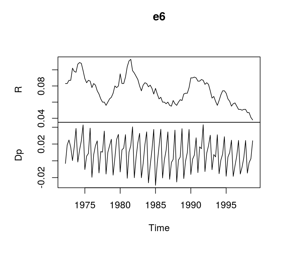

Estimation

There are multiple ways to estimate VEC models. A first approach would be to use ordinary least squares, which yields accurate result, but does not allow to estimate the cointegrating relations among the variables. The estimated generalised least squares (EGLS) approach would be an alternative. However, the most popular estimator for VECMs seems to be the maximum likelihood estimator of Johansen (1995), which is implemented in R by the ca.jo function of the urca package of Pfaff (2008a). Alternatively, function VECM of the tsDyn package of Di Narzo et al. (2020) can be used as well.¹

But before the VEC model can be estimated, the lag order $p$, the rank of the cointegration matrix $r$ and deterministic terms have to be specified. A valid strategy to choose the lag order is to estimated the VAR in levels and choose the lag specification that minimises an Information criterion. Since the time series show strong seasonal pattern, we control for this by specifying season = 4, where 4 is the frequency of the data.

library(vars) # Load package

# Estimate VAR
var_aic <- VAR(e6, type = "const", lag.max = 8, ic = "AIC", season = 4)

# Lag order suggested by AIC
var_aic$p

## AIC(n) 
##      4

According to the AIC, a lag order of 4 can be used, which is the same value used in Lütkepohl (2007). This means the VEC model corresponding to the VAR in levels has 3 lags. Since the ca.jo function requires the lag order of the VAR model we set K = 4.²

The inclusion of deterministic terms in a VECM is a delicate issue. Without going into detail a common strategy is to add a linear trend to the error correction term and a constant to the non-cointegration part of the equation. For this example we follow Lütkepohl (2007) and add a constant term and seasonal dummies to the non-cointegration part of the equation.

The ca.jo function does not just estimate the VECM. It also calculates the test statistics for different specificaions of $r$ and the user can choose between two alternative approaches, the trace and the eigenvalue test. For this example the trace test is used, i.e. type = "trace".

By default, the ca.jo function sets spec = "longrun" This specification would mean that the error correction term does not refer to the first lag of the variables in levels as decribed above, but to the $p-1$th lag instead. By setting spec = "transitory" the first lag will be used instead. Further information on the interpretation the two alternatives can be found in the function’s documentation ?ca.jo.

For further details on VEC modelling I recommend Lütkepohl (2006, Chapters 6, 7 and 8).

library(urca) # Load package

# Estimate
vec <- ca.jo(e6, ecdet = "none", type = "trace",
             K = 4, spec = "transitory", season = 4)

summary(vec)

## 
## ###################### 
## # Johansen-Procedure # 
## ###################### 
## 
## Test type: trace statistic , with linear trend 
## 
## Eigenvalues (lambda):
## [1] 0.15184737 0.03652339
## 
## Values of teststatistic and critical values of test:
## 
##           test 10pct  5pct  1pct
## r <= 1 |  3.83  6.50  8.18 11.65
## r = 0  | 20.80 15.66 17.95 23.52
## 
## Eigenvectors, normalised to first column:
## (These are the cointegration relations)
## 
##            R.l1    Dp.l1
## R.l1   1.000000 1.000000
## Dp.l1 -3.961937 1.700513
## 
## Weights W:
## (This is the loading matrix)
## 
##            R.l1       Dp.l1
## R.d  -0.1028717 -0.03938511
## Dp.d  0.1577005 -0.02146119

The trace test suggests that $r=1$ and the first columns of the estimates of the cointegration relations $\beta$ and the loading matrix $\alpha$ correspond to the results of the ML estimator in Lütkepohl (2007, Ch. 7):

# Beta
round(vec@V, 2)

##        R.l1 Dp.l1
## R.l1   1.00   1.0
## Dp.l1 -3.96   1.7

# Alpha
round(vec@W, 2)

##       R.l1 Dp.l1
## R.d  -0.10 -0.04
## Dp.d  0.16 -0.02

However, the estimated coefficients of the non-cointegration part of the model correspond to the results of the EGLS estimator.

round(vec@GAMMA, 2)

##      constant  sd1  sd2  sd3 R.dl1 Dp.dl1 R.dl2 Dp.dl2 R.dl3 Dp.dl3
## R.d      0.01 0.01 0.00 0.00  0.29  -0.16  0.01  -0.19  0.25  -0.09
## Dp.d    -0.01 0.02 0.02 0.03  0.08  -0.31  0.01  -0.37  0.04  -0.34

The deterministic terms are different from the results in Lütkepohl (2006), because different reference dates are used.

Using the the tsDyn package, estimates of the coefficients can be obtained in the following way:

# Load package
library(tsDyn)

# Obtain constant and seasonal dummies
seas <- gen_vec(data = e6, p = 4, r = 1, const = "unrestricted", seasonal = "unrestricted")
# Lag order p is 4 since gen_vec assumes that p corresponds to VAR form
seas <- seas$data$X[, 7:10]

# Estimate
est_tsdyn <- VECM(e6, lag = 3, r = 1, include = "none", estim = "ML", exogen = seas)

# Print results
summary(est_tsdyn)

## #############
## ###Model VECM 
## #############
## Full sample size: 107    End sample size: 103
## Number of variables: 2   Number of estimated slope parameters 22
## AIC -2142.333    BIC -2081.734   SSR 0.005033587
## Cointegrating vector (estimated by ML):
##    R        Dp
## r1 1 -3.961937
## 
## 
##             ECT                R -1               Dp -1              
## Equation R  -0.1029(0.0471)*   0.2688(0.1062)*    -0.2102(0.1581)    
## Equation Dp 0.1577(0.0445)***  0.0654(0.1003)     -0.3392(0.1493)*   
##             R -2                Dp -2              R -3              
## Equation R  -0.0178(0.1069)     -0.2230(0.1276).   0.2228(0.1032)*   
## Equation Dp -0.0043(0.1010)     -0.3908(0.1205)**  0.0184(0.0975)    
##             Dp -3               const              season.1          
## Equation R  -0.1076(0.0855)     0.0015(0.0038)     0.0015(0.0051)    
## Equation Dp -0.3472(0.0808)***  0.0102(0.0036)**   -0.0341(0.0048)***
##             season.2           season.3           
## Equation R  0.0089(0.0053).    -0.0004(0.0051)    
## Equation Dp -0.0179(0.0050)*** -0.0164(0.0048)***

Impulse response analyis

The impulse response function of a VECM is usually obtained from its VAR form. The function vec2var of the vars package can be used to transform the output of the ca.jo function into an object that can be handled by the irf function of the vars package. Note that since ur.jo does not set the rank $r$ of the cointegration matrix automatically, it has to be specified manually.

# Transform VEC to VAR with r = 1
var <- vec2var(vec, r = 1)

The impulse response function is then calculated in the usual manner by using the irf function.

# Obtain IRF
ir <- irf(var, n.ahead = 20, impulse = "R", response = "Dp",
          ortho = FALSE, runs = 500)

# Plot
plot(ir)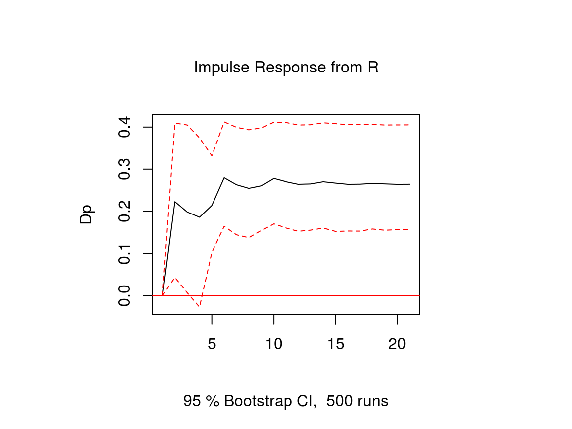

Note that an important difference to stationary VAR models is that the impulse response of a cointegrated VAR model does not neccessarily approach zero, because the variables are not stationary.

References

Lütkepohl, H. (2006). New introduction to multiple time series analysis (2nd ed.). Berlin: Springer.

Di Narzo, A. F., Aznarte, J. L., Stigler, M., &and Tsung-wu, H. (2020). tsDyn: Nonlinear Time Series Models with Regime Switching. R package version 10-1.2. https://CRAN.R-project.org/package=tsDyn

Pfaff, B. (2008a). Analysis of Integrated and Cointegrated Time Series with R. Second Edition. New York: Springer.

Pfaff, B. (2008b). VAR, SVAR and SVEC Models: Implementation Within R Package vars. Journal of Statistical Software 27(4).

Источник

Vector Error Correction Mechanism (VECM) models are a special application of VAR or Vector Autoregressive Models. The specification of VECM models involves the introduction of error correction terms into the VAR models. VECM methodology is used if the variables in the system have a long-run relationship, that is, they are cointegrated.

Every VAR model can be specified in the form of VECM by differencing the variables and introducing error correction terms. However, VECM is used only in the presence of cointegrating or long-run relationships. If there is no cointegration or if the variables are stationary, the VAR model should be applied. You can learn more about the interpretation of the VECM model in the VECM Estimation and Interpretation post.

Cointegration

Non-stationary variables are said to be cointegrated if their linear combination is stationary. For example, if two variables in a system are I(1) or integrated of order 1, but their linear regression yields an error term that is stationary. In such a case, we can say that the two variables are cointegrated and have a long-run relationship. Such variables move together over time and share a common stochastic trend. You can learn more about it from the post on Cointegration: Meaning, Tests and Models.

The VECM model is used to analyze cointegrated variables or cointegrating relationships. It provides a mechanism to understand the long-run as well as short-run behaviour of the variables in the system.

Vector Error Correction: Underlying VAR model

As stated earlier, every VAR model can be expressed in the form of VECM using differences and error correction terms. This also implies that every VECM model has an underlying VAR model. To understand the specification of VECM, we must look at the underlying VAR model specification.

Any VAR model can be specified in the matrix form as follows:

In VAR and VECM terminology, the error terms are referred to as impulses or innovations. To illustrate further, let us consider a VAR model with 2 variables and 3 lags:

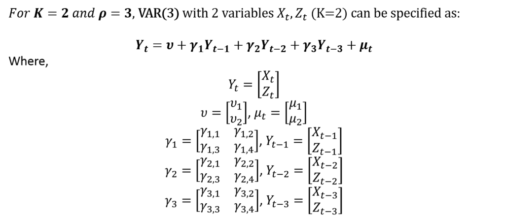
This VAR(3) with 2 variables (K = 2) is in the matrix form. The appropriate lags (p) must be chosen with the help of Information Criteria. Moreover, the number of lags must ensure that there is no autocorrelation.

Cointegration and Vector Error Correction Mechanism (VECM)

The VECM models are specified in differences to account for short-run behaviour. Along with the short-run, VECM models include error correction terms and cointegrating equations to account for short-run adjustments and long-run cointegrating relationships. The general form of a VECM can be specified as:

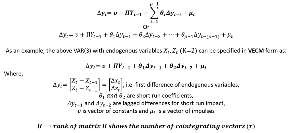
In the example, we can compare the VAR and VECM specifications for K = 2 model. The underlying VAR model has 3 lags, whereas, its VECM specification has 2 lags of differences. Therefore, the VECM form has one less lag (p – 1 lags) as compared to the underlying VAR model.

The Rank of the coefficient matrix associated with Y_t-1 shows the number of cointegrating vectors (“r”). The number of cointegrating or long-run relationships (r) can be determined using Johansen’s Test of Cointegration.

Choosing between VAR and VECM

Tests of cointegration must be applied to ascertain whether the system of variables has any cointegrating relationships. Usually, Johansen’s Test of Cointegration is used to check for cointegration. Johansen provided a framework to check for cointegrating relationships and apply the Vector Error Correction Mechanism (VECM) to estimate short-run coefficients, short-run adjustment coefficients and long-run cointegrating relationships.

Using Johansen’s Test of Cointegration, we can determine “r”, which is the number of cointegrating vectors. In a system of “K” variables, there are 3 different scenarios:

Number of cointegrating vectors (r)	Meaning	Stationarity of variables	Model to be used	Results
r = 0	No cointegration	The variables are non-stationary and there are no long-run relationships among them	Apply VAR in differences	the VAR results show short-run coefficients
0 < r < K	Cointegration exists	The variables are non-stationary and the number of cointegrating relationships is equal to “r”	Apply VECM	The VECM results show short-run coefficients and long-run equilibrium/cointegration relationship
r = K	No cointegration	The variables are stationary and cointegration cannot exist in stationary variables	Apply VAR to variables in their original form	The VAR results show long-run coefficients because the variables are not in differences

Suppose, we determine that cointegration exists (0 < r < K) using Johansen’s Test of Cointegration. Then, we can specify the above VECM model as:

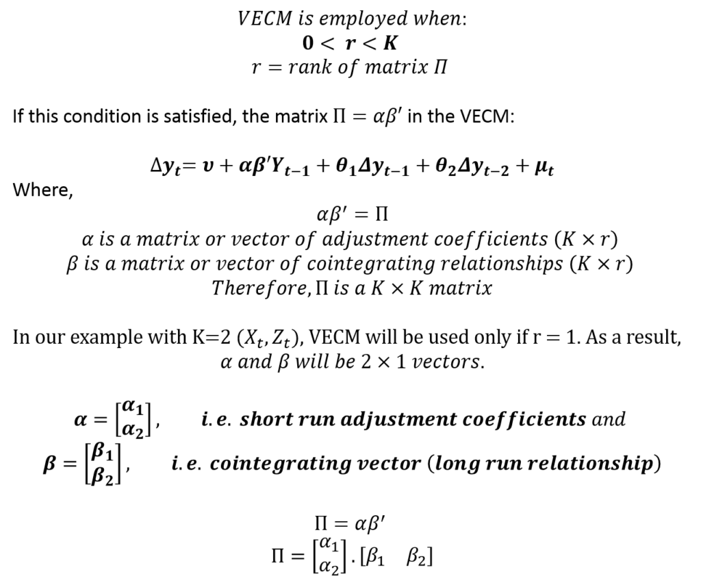
Hence, the VECM model gives us estimates of short-run behaviour, long-run cointegrating relationship as well as short-run adjustment coefficients. The short-run deviations from long-run equilibrium are corrected and the speed of this correction is shown by the adjustment coefficients.

The framework developed by Johansen allows the inclusion of several types of trends and constants in the short-run equations as well as in the cointegrating relationships. The specification of trends and constants differ according to the data. Some preliminary analysis is needed to determine the appropriate trend specifications. Let us consider all the trend specifications allowed under Johansen’s framework and when to employ them.

Specification of trends in VECM

Case 1: Unrestricted Trend

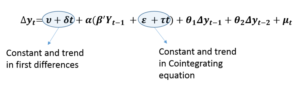
Firstly, an Unrestricted trend in a VECM means that we include a constant and a trend in the cointegrating equations as well as in the first differences. This specification implies a quadratic trend in the levels of variables because we are including a trend term in the first differences. Hence, this model should be used only if the variables show a quadratic trend. It is essential to plot the variables on a graph to check for quadratic trends or do formal testing for quadratic trends in the data.

The cointegrating equations are stationary around a time trend, that is, they are trend stationary. Hence, this specification allows the cointegrating equations to be trend stationary and original variables to have a quadratic trend.

Case 2: Restricted Trend

Secondly, Restricted trend specification does not include a trend in first differences, which implies a linear trend in original variables. In addition, it allows the cointegrating equations to be trend stationary. Hence, this specification should be used when the levels of variables have a linear trend and the cointegrating equations are stationary around a time trend, i.e. trend stationary.

In practice, a linear trend is easy to recognise. But, the trend stationarity of the cointegrating equations can be analyzed only after estimating the VECM. Therefore, it is advisable to estimate this model and then check whether a trend coefficient is needed in the cointegrating relationships or not.

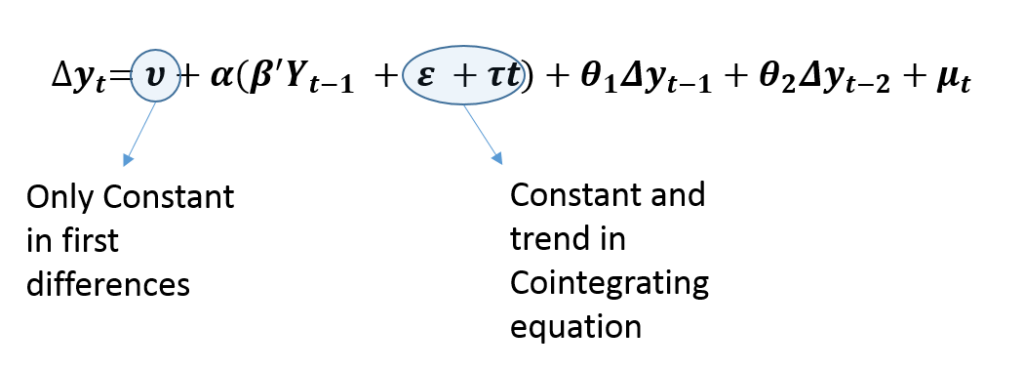
Case 3: Unrestricted Constant

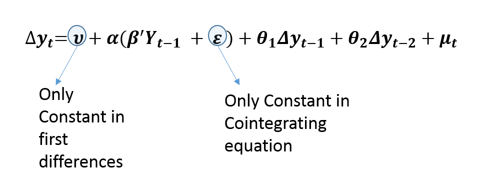
Thirdly, Unrestricted Constant is the most commonly used specification of VECM. Similar to the Restricted trend, it allows a linear trend in original or levels of variables. This is evident from the fact that we include only the constant term in the first differences. However, it is different from the Restricted trend specification because it includes only a constant in cointegrating relationships.

This specification allows the cointegrating or long-run relationship to be stationary around some constant mean. Hence, there is no trend in cointegrating relationships. As a result, it is used when there is a linear trend in original variables along with a cointegrating relationship that is stationary around some non-zero mean.

Case 4: Restricted Constant

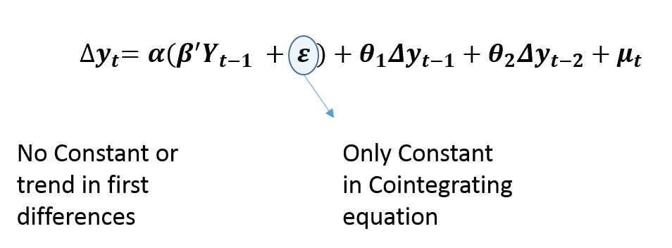
Restricted Constant specification does not include a constant or a trend in first differences. This implies that there is no trend in the levels of variables. It only allows a constant in the cointegrating relationships, meaning that it is stationary around a constant mean. This specification is used when the original variables do not show any linear trends and the cointegrating relationships are stationary around a constant mean without any trend.

Case 5: No Trend

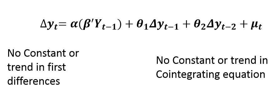
Finally, this specification of no trend is rarely used in practice. It does not include any trend or constant terms in the VECM model. It implies that the levels of variables show no trend and have zero means. Moreover, the cointegrating relationships are stationary around zero mean.

Источник

Векторные модели исправления ошибок

Многомерные линейные модели включая cointegrating отношения и внешние переменные предикторы

Модели векторного исправления ошибок (VEC) или cointegrated VAR models, обращаются к нестационарности в многомерном временном ряду, следующем из co-перемещений ряда множественного ответа. Для примера анализа с помощью инструментов моделирования VEC смотрите Моделирование Экономики Соединенных Штатов.

Функции

развернуть все

Создайте модель

vecm Создайте модель векторного исправления ошибок (VEC)

Подбирайте модель к данным

`estimate`	Подбирайте модель векторного исправления ошибок (VEC) к данным
`infer`	Выведите инновации модели векторного исправления ошибок (VEC)
`summarize`	Отобразите результаты оценки модели векторного исправления ошибок (VEC)

Преобразуйте между моделями

`arma2ar`	Преобразуйте модель ARMA в модель AR
`arma2ma`	Преобразуйте модель ARMA в модель MA
`vec2var`	Преобразуйте модель VEC в модель VAR
`var2vec`	Преобразуйте модель VAR в модель VEC
`varm`	Преобразуйте модель векторного исправления ошибок (VEC) в векторную модель (VAR) авторегрессии

Сгенерируйте симуляции или импульсные характеристики

`simulate`	Симуляция Монте-Карло модели векторного исправления ошибок (VEC)
`filter`	Пропустите воздействия через модель векторного исправления ошибок (VEC)
`irf`	Сгенерируйте импульсные характеристики модели векторного исправления ошибок (VEC)
`fevd`	Сгенерируйте разложение отклонения ошибки прогноза (FEVD) модели векторного исправления ошибок (VEC)

Сгенерируйте минимальные прогнозы среднеквадратичной погрешности

forecast Предскажите ответы модели векторного исправления ошибок (VEC)

Темы

Источник

History[edit]

Estimation[edit]

Engle and Granger 2-step approach[edit]

VECM[edit]

An example of ECM[edit]

References[edit]

Further reading[edit]

Векторная модель коррекции ошибок

Model and data

Estimation

Impulse response analyis

References

Cointegration

Vector Error Correction: Underlying VAR model

Cointegration and Vector Error Correction Mechanism (VECM)

Choosing between VAR and VECM

Specification of trends in VECM

Case 1: Unrestricted Trend

Case 2: Restricted Trend

Case 3: Unrestricted Constant

Case 4: Restricted Constant

Case 5: No Trend

Векторные модели исправления ошибок

Функции

Создайте модель

Подбирайте модель к данным

Преобразуйте между моделями

Сгенерируйте симуляции или импульсные характеристики

Сгенерируйте минимальные прогнозы среднеквадратичной погрешности

Темы