В корреляционно-регрессионном
анализе обычно оценивается достоверность
не только уравнения в целом, но и отдельных
параметров связи. Статистическая
оценка выборочного коэффициента
корреляции, как и других параметров,
проводится только в том случае, если
выборочная совокупность формировалась
в случайном порядке. Алгоритм оценки
достоверности выборочных коэффициентов
корреляции предусматривает расчет
критериев достоверности t-Стьюдента
(для малых выборок) и t-нормального
распределения (для больших выборок) как
отношения выборочного коэффициента
корреляции к его средней ошибке
tr
=
![]()
3.5.
Средняя или
стандартная ошибка коэффициента
корреляции mr
покажет,
на какую величину в среднем по всем
возможным выборкам равного объема
выборочные коэффициенты корреляции
(оценки) r
будут отличаться от истинного
(генерального) коэффициента корреляции
![]()
.
Величина
стандартной ошибки коэффициента
корреляции в случае парной линейной
связи определяется по формуле
![]()
3.6.
Тогда фактическое
значение t-критерия
определяется как
![]()
3.7.
Сравнив полученное
фактическое значение критерия с его
критическим (табличным) значением, можно
сделать вывод о достоверности выборочного
коэффициента корреляции.
Например, по
результатам случайной выборки семей
(п
= 20) был определен выборочный коэффициент
корреляции между доходом семьи и
потреблением товара А: ryx
= 0,88.
а) Выдвинем нулевую
гипотезу, что данная величина выборочного
коэффициента корреляции явилась
следствием случайных колебаний выборочных
данных, на основании которых он исчислен,
а генеральный коэффициент корреляции
равен нулю – Н0:
=0.
б) Определим среднюю
ошибку выборочного коэффициента
корреляции :
=![]()
в) Рассчитаем
фактическое значение критерия t
–Стьюдента:
tr
=
=![]()
.
г) По таблице
значений критерия t
–Стьюдента определим его критическое
значение при уровне значимости 0,05 и
числе степеней свободы dfост
= п-2=18:
tst
= 2,1009.
д ) Сопоставим
критическое и фактическое значения
критерия Стьюдента: tфакт.>
tst
(7,86>2,1009).
Сделаем вывод.
С вероятностью
0,95 мы отвергаем нулевую гипотезу
о равенстве коэффициента корреляции
в генеральной совокупности нулю.
Выборочный
показатель связи обеспечивает точечную
оценку рассматриваемого параметра, но
при этом вероятность того, что истинное
значение будет в точности равно этой
оценке, ничтожно мала. Доверительный
интервал дает так называемую интервальную
оценку параметра, то есть диапазон
значений, который будет включать истинное
значение с высокой, заранее определенной
вероятностью. Для расчета доверительного
интервала необходимо найти предельную
ошибку коэффициента корреляции по
формуле
![]()
=
tst
∙mr
=
2,1009∙0,112=0,235.
Предельная ошибка покажет, на какую
максимальную величину для данного
уровня вероятности выборочный коэффициент
корреляции может отличаться от
генерального.
Доверительный
интервал для коэффициента корреляции
определяется как
![]()
3.8.
для нашего примера:
0,88 -0,235![]()
0,88
+ 0,235. Учитывая,
что коэффициент корреляции принимает
значения от 0 до 1, сделаем вывод:
с уровнем вероятности
0,95 можно утверждать, что коэффициент
корреляции между доходом семьи и
потреблением товара А в генеральной
совокупности находится в интервале от
0,645 до 1.
Соседние файлы в предмете [НЕСОРТИРОВАННОЕ]
- #
- #
- #
- #
- #
- #
- #
- #
- #
- #
- #
In statistics, the Pearson correlation coefficient (PCC, pronounced ) ― also known as Pearson’s r, the Pearson product-moment correlation coefficient (PPMCC), the bivariate correlation,[1] or colloquially simply as the correlation coefficient[2] ― is a measure of linear correlation between two sets of data. It is the ratio between the covariance of two variables and the product of their standard deviations; thus, it is essentially a normalized measurement of the covariance, such that the result always has a value between −1 and 1. As with covariance itself, the measure can only reflect a linear correlation of variables, and ignores many other types of relationships or correlations. As a simple example, one would expect the age and height of a sample of teenagers from a high school to have a Pearson correlation coefficient significantly greater than 0, but less than 1 (as 1 would represent an unrealistically perfect correlation).
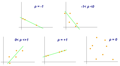
Examples of scatter diagrams with different values of correlation coefficient (ρ)
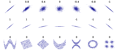
Several sets of (x, y) points, with the correlation coefficient of x and y for each set. Note that the correlation reflects the strength and direction of a linear relationship (top row), but not the slope of that relationship (middle), nor many aspects of nonlinear relationships (bottom). N.B.: the figure in the center has a slope of 0 but in that case the correlation coefficient is undefined because the variance of Y is zero.
Naming and history[edit]
It was developed by Karl Pearson from a related idea introduced by Francis Galton in the 1880s, and for which the mathematical formula was derived and published by Auguste Bravais in 1844.[a][6][7][8][9] The naming of the coefficient is thus an example of Stigler’s Law.
Definition[edit]
Pearson’s correlation coefficient is the covariance of the two variables divided by the product of their standard deviations. The form of the definition involves a «product moment», that is, the mean (the first moment about the origin) of the product of the mean-adjusted random variables; hence the modifier product-moment in the name.
For a population[edit]
Pearson’s correlation coefficient, when applied to a population, is commonly represented by the Greek letter ρ (rho) and may be referred to as the population correlation coefficient or the population Pearson correlation coefficient. Given a pair of random variables  , the formula for ρ[10] is:[11]

where:
The formula for  can be expressed in terms of mean and expectation. Since[10]
![{displaystyle operatorname {cov} (X,Y)=operatorname {mathbb {E} } [(X-mu _{X})(Y-mu _{Y})],}](https://wikimedia.org/api/rest_v1/media/math/render/svg/1e88bc4ba085b98d5cca09b958ad378d50127308)
the formula for can also be written as
![{displaystyle rho _{X,Y}={frac {operatorname {mathbb {E} } [(X-mu _{X})(Y-mu _{Y})]}{sigma _{X}sigma _{Y}}}}](https://wikimedia.org/api/rest_v1/media/math/render/svg/042c646e848d2dc6e15d7b5c7a5b891941b2eab6)
where:
The formula for can be expressed in terms of uncentered moments. Since
![{displaystyle mu _{X}=operatorname {mathbb {E} } [,X,]}](https://wikimedia.org/api/rest_v1/media/math/render/svg/1182bdcc66a113596e3ece07a0acbeda8d56d483)
![{displaystyle mu _{Y}=operatorname {mathbb {E} } [,Y,]}](https://wikimedia.org/api/rest_v1/media/math/render/svg/b2f14f5eda9d726e57048a2c56889912a80a06b6)
![{displaystyle sigma _{X}^{2}=operatorname {mathbb {E} } [,left(X-operatorname {mathbb {E} } [X]right)^{2},]=operatorname {mathbb {E} } [,X^{2},]-left(operatorname {mathbb {E} } [,X,]right)^{2}}](https://wikimedia.org/api/rest_v1/media/math/render/svg/cbf27c91550c7c82ee7e9e948673eb99da1a7378)
![{displaystyle sigma _{Y}^{2}=operatorname {mathbb {E} } [,left(Y-operatorname {mathbb {E} } [Y]right)^{2},]=operatorname {mathbb {E} } [,Y^{2},]-left(,operatorname {mathbb {E} } [,Y,]right)^{2}}](https://wikimedia.org/api/rest_v1/media/math/render/svg/ed498483dae15dbb86e957b5a1463f5536885902)
![{displaystyle operatorname {mathbb {E} } [,left(X-mu _{X}right)left(Y-mu _{Y}right),]=operatorname {mathbb {E} } [,left(X-operatorname {mathbb {E} } [,X,]right)left(Y-operatorname {mathbb {E} } [,Y,]right),]=operatorname {mathbb {E} } [,X,Y,]-operatorname {mathbb {E} } [,X,]operatorname {mathbb {E} } [,Y,],,}](https://wikimedia.org/api/rest_v1/media/math/render/svg/4443378e105084380438782ebd391f8cb0e8e048)
the formula for can also be written as
![{displaystyle rho _{X,Y}={frac {operatorname {mathbb {E} } [,X,Y,]-operatorname {mathbb {E} } [,X,]operatorname {mathbb {E} } [,Y,]}{{sqrt {operatorname {mathbb {E} } [,X^{2},]-left(operatorname {mathbb {E} } [,X,]right)^{2}}}~{sqrt {operatorname {mathbb {E} } [,Y^{2},]-left(operatorname {mathbb {E} } [,Y,]right)^{2}}}}}.}](https://wikimedia.org/api/rest_v1/media/math/render/svg/0a96c914bb811b84698b4d4118794cf4c8167ca7)
Peason’s correlation coefficient does not exist when either  or
or  are zero, infinite or undefined.
For a sample[edit]
Pearson’s correlation coefficient, when applied to a sample, is commonly represented by  and may be referred to as the sample correlation coefficient or the sample Pearson correlation coefficient. We can obtain a formula for by substituting estimates of the covariances and variances based on a sample into the formula above. Given paired data
  consisting of
  pairs, is defined as:

where:
Rearranging gives us this formula for :

where  are defined as above.
This formula suggests a convenient single-pass algorithm for calculating sample correlations, though depending on the numbers involved, it can sometimes be numerically unstable.
Rearranging again gives us this[10] formula for :

where  are defined as above.
An equivalent expression gives the formula for as the mean of the products of the standard scores as follows:

where:
Alternative formulae for are also available. For example, one can use the following formula for :

where:
Practical issues[edit]
Under heavy noise conditions, extracting the correlation coefficient between two sets of stochastic variables is nontrivial, in particular where Canonical Correlation Analysis reports degraded correlation values due to the heavy noise contributions. A generalization of the approach is given elsewhere.[12]
In case of missing data, Garren derived the maximum likelihood estimator.[13]
Some distributions (e.g., stable distributions other than a normal distribution) do not have a defined variance.
Mathematical properties[edit]
The values of both the sample and population Pearson correlation coefficients are on or between −1 and 1. Correlations equal to +1 or −1 correspond to data points lying exactly on a line (in the case of the sample correlation), or to a bivariate distribution entirely supported on a line (in the case of the population correlation). The Pearson correlation coefficient is symmetric: corr(X,Y) = corr(Y,X).
A key mathematical property of the Pearson correlation coefficient is that it is invariant under separate changes in location and scale in the two variables. That is, we may transform X to a + bX and transform Y to c + dY, where a, b, c, and d are constants with b, d > 0, without changing the correlation coefficient. (This holds for both the population and sample Pearson correlation coefficients.) Note that more general linear transformations do change the correlation: see § Decorrelation of n random variables for an application of this.
Interpretation[edit]
The correlation coefficient ranges from −1 to 1. An absolute value of exactly 1 implies that a linear equation describes the relationship between X and Y perfectly, with all data points lying on a line. The correlation sign is determined by the regression slope: a value of +1 implies that all data points lie on a line for which Y increases as X increases, and vice versa for −1.[14] A value of 0 implies that there is no linear dependency between the variables.[15]
More generally, note that (Xi − X)(Yi − Y) is positive if and only if Xi and Yi lie on the same side of their respective means. Thus the correlation coefficient is positive if Xi and Yi tend to be simultaneously greater than, or simultaneously less than, their respective means. The correlation coefficient is negative (anti-correlation) if Xi and Yi tend to lie on opposite sides of their respective means. Moreover, the stronger either tendency is, the larger is the absolute value of the correlation coefficient.
Rodgers and Nicewander[16] cataloged thirteen ways of interpreting correlation or simple functions of it:
- Function of raw scores and means
- Standardized covariance
- Standardized slope of the regression line
- Geometric mean of the two regression slopes
- Square root of the ratio of two variances
- Mean cross-product of standardized variables
- Function of the angle between two standardized regression lines
- Function of the angle between two variable vectors
- Rescaled variance of the difference between standardized scores
- Estimated from the balloon rule
- Related to the bivariate ellipses of isoconcentration
- Function of test statistics from designed experiments
- Ratio of two means
Geometric interpretation[edit]
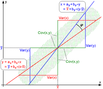
Regression lines for y = gX(x) [red] and x = gY(y) [blue]
For uncentered data, there is a relation between the correlation coefficient and the angle φ between the two regression lines, y = gX(x) and x = gY(y), obtained by regressing y on x and x on y respectively. (Here, φ is measured counterclockwise within the first quadrant formed around the lines’ intersection point if r > 0, or counterclockwise from the fourth to the second quadrant if r < 0.) One can show[17] that if the standard deviations are equal, then r = sec φ − tan φ, where sec and tan are trigonometric functions.
For centered data (i.e., data which have been shifted by the sample means of their respective variables so as to have an average of zero for each variable), the correlation coefficient can also be viewed as the cosine of the angle θ between the two observed vectors in N-dimensional space (for N observations of each variable)[18]
Both the uncentered (non-Pearson-compliant) and centered correlation coefficients can be determined for a dataset. As an example, suppose five countries are found to have gross national products of 1, 2, 3, 5, and 8 billion dollars, respectively. Suppose these same five countries (in the same order) are found to have 11%, 12%, 13%, 15%, and 18% poverty. Then let x and y be ordered 5-element vectors containing the above data: x = (1, 2, 3, 5, and y = (0.11, 0.12, 0.13, 0.15, 0.18).
By the usual procedure for finding the angle θ between two vectors (see dot product), the uncentered correlation coefficient is:

This uncentered correlation coefficient is identical with the cosine similarity.
Note that the above data were deliberately chosen to be perfectly correlated: y = 0.10 + 0.01 x. The Pearson correlation coefficient must therefore be exactly one. Centering the data (shifting x by ℰ(x) = 3.8 and y by ℰ(y) = 0.138) yields x = (−2.8, −1.8, −0.8, 1.2, 4.2) and y = (−0.028, −0.018, −0.008, 0.012, 0.042), from which

as expected.
Interpretation of the size of a correlation[edit]
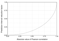
This figure gives a sense of how the usefulness of a Pearson correlation for predicting values varies with its magnitude. Given jointly normal X, Y with correlation ρ,  (plotted here as a function of ρ) is the factor by which a given prediction interval for Y may be reduced given the corresponding value of X. For example, if ρ = 0.5, then the 95% prediction interval of Y|X will be about 13% smaller than the 95% prediction interval of Y.
Several authors have offered guidelines for the interpretation of a correlation coefficient.[19][20] However, all such criteria are in some ways arbitrary.[20] The interpretation of a correlation coefficient depends on the context and purposes. A correlation of 0.8 may be very low if one is verifying a physical law using high-quality instruments, but may be regarded as very high in the social sciences, where there may be a greater contribution from complicating factors.
Inference[edit]
Statistical inference based on Pearson’s correlation coefficient often focuses on one of the following two aims:
- One aim is to test the null hypothesis that the true correlation coefficient ρ is equal to 0, based on the value of the sample correlation coefficient r.
- The other aim is to derive a confidence interval that, on repeated sampling, has a given probability of containing ρ.
We discuss methods of achieving one or both of these aims below.
Using a permutation test[edit]
Permutation tests provide a direct approach to performing hypothesis tests and constructing confidence intervals. A permutation test for Pearson’s correlation coefficient involves the following two steps:
- Using the original paired data (xi, yi), randomly redefine the pairs to create a new data set (xi, yi′), where the i′ are a permutation of the set {1,…,n}. The permutation i′ is selected randomly, with equal probabilities placed on all n! possible permutations. This is equivalent to drawing the i′ randomly without replacement from the set {1, …, n}. In bootstrapping, a closely related approach, the i and the i′ are equal and drawn with replacement from {1, …, n};
- Construct a correlation coefficient r from the randomized data.
To perform the permutation test, repeat steps (1) and (2) a large number of times. The p-value for the permutation test is the proportion of the r values generated in step (2) that are larger than the Pearson correlation coefficient that was calculated from the original data. Here «larger» can mean either that the value is larger in magnitude, or larger in signed value, depending on whether a two-sided or one-sided test is desired.
Using a bootstrap[edit]
The bootstrap can be used to construct confidence intervals for Pearson’s correlation coefficient. In the «non-parametric» bootstrap, n pairs (xi, yi) are resampled «with replacement» from the observed set of n pairs, and the correlation coefficient r is calculated based on the resampled data. This process is repeated a large number of times, and the empirical distribution of the resampled r values are used to approximate the sampling distribution of the statistic. A 95% confidence interval for ρ can be defined as the interval spanning from the 2.5th to the 97.5th percentile of the resampled r values.
Standard error[edit]
If  and
and  are random variables, a standard error associated to the correlation in the null case is:

where  is the correlation (assumed r≈0) and the sample size.[21][22]
Testing using Student’s t-distribution[edit]
Critical values of Pearson’s correlation coefficient that must be exceeded to be considered significantly nonzero at the 0.05 level.
For pairs from an uncorrelated bivariate normal distribution, the sampling distribution of the studentized Pearson’s correlation coefficient follows Student’s t-distribution with degrees of freedom n − 2. Specifically, if the underlying variables have a bivariate normal distribution, the variable

has a student’s t-distribution in the null case (zero correlation).[23] This holds approximately in case of non-normal observed values if sample sizes are large enough.[24] For determining the critical values for r the inverse function is needed:

Alternatively, large sample, asymptotic approaches can be used.
Another early paper[25] provides graphs and tables for general values of ρ, for small sample sizes, and discusses computational approaches.
In the case where the underlying variables are not normal, the sampling distribution of Pearson’s correlation coefficient follows a Student’s t-distribution, but the degrees of freedom are reduced.[26]
Using the exact distribution[edit]
For data that follow a bivariate normal distribution, the exact density function f(r) for the sample correlation coefficient r of a normal bivariate is[27][28][29]

where  is the gamma function and
  is the Gaussian hypergeometric function.
In the special case when  (zero population correlation), the exact density function f(r) can be written as:

where  is the beta function, which is one way of writing the density of a Student’s t-distribution, as above.
Using the exact confidence distribution[edit]
Confidence intervals and tests can be calculated from a confidence distribution. An exact confidence density for ρ is[30]

where  is the Gaussian hypergeometric function and
  .
.
Using the Fisher transformation[edit]
In practice, confidence intervals and hypothesis tests relating to ρ are usually carried out using the Fisher transformation, :

F(r) approximately follows a normal distribution with
 and standard error


where n is the sample size. The approximation error is lowest for a large sample size and small and  and increases otherwise.
Using the approximation, a z-score is
![z={frac {x-{text{mean}}}{text{SE}}}=[F(r)-F(rho _{0})]{sqrt {n-3}}](https://wikimedia.org/api/rest_v1/media/math/render/svg/da7a3d54a70f9005e3bf9a2accf62cbf0fa0ea71)
under the null hypothesis that  , given the assumption that the sample pairs are independent and identically distributed and follow a bivariate normal distribution. Thus an approximate p-value can be obtained from a normal probability table. For example, if z = 2.2 is observed and a two-sided p-value is desired to test the null hypothesis that , the p-value is 2 Φ(−2.2) = 0.028, where Φ is the standard normal cumulative distribution function.
To obtain a confidence interval for ρ, we first compute a confidence interval for F():
![{displaystyle 100(1-alpha )%{text{CI}}:operatorname {artanh} (rho )in [operatorname {artanh} (r)pm z_{alpha /2}{text{SE}}]}](https://wikimedia.org/api/rest_v1/media/math/render/svg/affc3f0ee39499c97bb851229113f49d83100bf2)
The inverse Fisher transformation brings the interval back to the correlation scale.
![{displaystyle 100(1-alpha )%{text{CI}}:rho in [tanh(operatorname {artanh} (r)-z_{alpha /2}{text{SE}}),tanh(operatorname {artanh} (r)+z_{alpha /2}{text{SE}})]}](https://wikimedia.org/api/rest_v1/media/math/render/svg/bf658969d39ea848505750b5cd76db21da78dd5c)
For example, suppose we observe r = 0.7 with a sample size of n=50, and we wish to obtain a 95% confidence interval for ρ. The transformed value is arctanh(r) = 0.8673, so the confidence interval on the transformed scale is 0.8673 ± 1.96/√47, or (0.5814, 1.1532). Converting back to the correlation scale yields (0.5237, 0.8188).
In least squares regression analysis[edit]
The square of the sample correlation coefficient is typically denoted r2 and is a special case of the coefficient of determination. In this case, it estimates the fraction of the variance in Y that is explained by X in a simple linear regression. So if we have the observed dataset  and the fitted dataset
  then as a starting point the total variation in the Yi around their average value can be decomposed as follows

where the  are the fitted values from the regression analysis. This can be rearranged to give

The two summands above are the fraction of variance in Y that is explained by X (right) and that is unexplained by X (left).
Next, we apply a property of least square regression models, that the sample covariance between and  is zero. Thus, the sample correlation coefficient between the observed and fitted response values in the regression can be written (calculation is under expectation, assumes Gaussian statistics)
![{displaystyle {begin{aligned}r(Y,{hat {Y}})&={frac {sum _{i}(Y_{i}-{bar {Y}})({hat {Y}}_{i}-{bar {Y}})}{sqrt {sum _{i}(Y_{i}-{bar {Y}})^{2}cdot sum _{i}({hat {Y}}_{i}-{bar {Y}})^{2}}}}[6pt]&={frac {sum _{i}(Y_{i}-{hat {Y}}_{i}+{hat {Y}}_{i}-{bar {Y}})({hat {Y}}_{i}-{bar {Y}})}{sqrt {sum _{i}(Y_{i}-{bar {Y}})^{2}cdot sum _{i}({hat {Y}}_{i}-{bar {Y}})^{2}}}}[6pt]&={frac {sum _{i}[(Y_{i}-{hat {Y}}_{i})({hat {Y}}_{i}-{bar {Y}})+({hat {Y}}_{i}-{bar {Y}})^{2}]}{sqrt {sum _{i}(Y_{i}-{bar {Y}})^{2}cdot sum _{i}({hat {Y}}_{i}-{bar {Y}})^{2}}}}[6pt]&={frac {sum _{i}({hat {Y}}_{i}-{bar {Y}})^{2}}{sqrt {sum _{i}(Y_{i}-{bar {Y}})^{2}cdot sum _{i}({hat {Y}}_{i}-{bar {Y}})^{2}}}}[6pt]&={sqrt {frac {sum _{i}({hat {Y}}_{i}-{bar {Y}})^{2}}{sum _{i}(Y_{i}-{bar {Y}})^{2}}}}.end{aligned}}}](https://wikimedia.org/api/rest_v1/media/math/render/svg/d86595f3f77e8ee96952760d9176a5fa140cc562)
Thus

where  is the proportion of variance in Y explained by a linear function of X.
In the derivation above, the fact that

can be proved by noticing that the partial derivatives of the residual sum of squares (RSS) over β0 and β1 are equal to 0 in the least squares model, where
- .

In the end, the equation can be written as:

where
The symbol  is called the regression sum of squares, also called the explained sum of squares, and
  is the total sum of squares (proportional to the variance of the data).
Sensitivity to the data distribution[edit]
Existence[edit]
The population Pearson correlation coefficient is defined in terms of moments, and therefore exists for any bivariate probability distribution for which the population covariance is defined and the marginal population variances are defined and are non-zero. Some probability distributions, such as the Cauchy distribution, have undefined variance and hence ρ is not defined if X or Y follows such a distribution. In some practical applications, such as those involving data suspected to follow a heavy-tailed distribution, this is an important consideration. However, the existence of the correlation coefficient is usually not a concern; for instance, if the range of the distribution is bounded, ρ is always defined.
Sample size[edit]
- If the sample size is moderate or large and the population is normal, then, in the case of the bivariate normal distribution, the sample correlation coefficient is the maximum likelihood estimate of the population correlation coefficient, and is asymptotically unbiased and efficient, which roughly means that it is impossible to construct a more accurate estimate than the sample correlation coefficient.
- If the sample size is large and the population is not normal, then the sample correlation coefficient remains approximately unbiased, but may not be efficient.
- If the sample size is large, then the sample correlation coefficient is a consistent estimator of the population correlation coefficient as long as the sample means, variances, and covariance are consistent (which is guaranteed when the law of large numbers can be applied).
- If the sample size is small, then the sample correlation coefficient r is not an unbiased estimate of ρ.[10] The adjusted correlation coefficient must be used instead: see elsewhere in this article for the definition.
- Correlations can be different for imbalanced dichotomous data when there is variance error in sample.[31]
Robustness[edit]
Like many commonly used statistics, the sample statistic r is not robust,[32] so its value can be misleading if outliers are present.[33][34] Specifically, the PMCC is neither distributionally robust,[citation needed] nor outlier resistant[32] (see Robust statistics § Definition). Inspection of the scatterplot between X and Y will typically reveal a situation where lack of robustness might be an issue, and in such cases it may be advisable to use a robust measure of association. Note however that while most robust estimators of association measure statistical dependence in some way, they are generally not interpretable on the same scale as the Pearson correlation coefficient.
Statistical inference for Pearson’s correlation coefficient is sensitive to the data distribution. Exact tests, and asymptotic tests based on the Fisher transformation can be applied if the data are approximately normally distributed, but may be misleading otherwise. In some situations, the bootstrap can be applied to construct confidence intervals, and permutation tests can be applied to carry out hypothesis tests. These non-parametric approaches may give more meaningful results in some situations where bivariate normality does not hold. However the standard versions of these approaches rely on exchangeability of the data, meaning that there is no ordering or grouping of the data pairs being analyzed that might affect the behavior of the correlation estimate.
A stratified analysis is one way to either accommodate a lack of bivariate normality, or to isolate the correlation resulting from one factor while controlling for another. If W represents cluster membership or another factor that it is desirable to control, we can stratify the data based on the value of W, then calculate a correlation coefficient within each stratum. The stratum-level estimates can then be combined to estimate the overall correlation while controlling for W.[35]
Variants[edit]
Variations of the correlation coefficient can be calculated for different purposes. Here are some examples.
Adjusted correlation coefficient[edit]
The sample correlation coefficient r is not an unbiased estimate of ρ. For data that follows a bivariate normal distribution, the expectation E[r] for the sample correlation coefficient r of a normal bivariate is[36]
- therefore r is a biased estimator of
![{displaystyle operatorname {mathbb {E} } left[rright]=rho -{frac {rho left(1-rho ^{2}right)}{2n}}+cdots ,quad }](https://wikimedia.org/api/rest_v1/media/math/render/svg/683b838e709e3b32a3c22dfec4fa665a593f42ad)

The unique minimum variance unbiased estimator radj is given by[37]
-
(1)

where:
An approximately unbiased estimator radj can be obtained[citation needed] by truncating E[r] and solving this truncated equation:
-
(2)
![{displaystyle r=operatorname {mathbb {E} } [r]approx r_{text{adj}}-{frac {r_{text{adj}}(1-r_{text{adj}}^{2})}{2n}}.}](https://wikimedia.org/api/rest_v1/media/math/render/svg/6382c40e3ad4e06d65c7d09e214ebc8daba5d30c)
An approximate solution[citation needed] to equation (2) is:
-
(3)
![{displaystyle r_{text{adj}}approx rleft[1+{frac {1-r^{2}}{2n}}right],}](https://wikimedia.org/api/rest_v1/media/math/render/svg/cbf3f71f2cfe17f8f0d422d5ac0d482cc429a925)
where in (3):
- are defined as above,
- radj is a suboptimal estimator,[citation needed][clarification needed]
- radj can also be obtained by maximizing log(f(r)),
- radj has minimum variance for large values of n,
- radj has a bias of order 1⁄(n − 1).

Another proposed[10] adjusted correlation coefficient is:[citation needed]

Note that radj ≈ r for large values of n.
Weighted correlation coefficient[edit]
Suppose observations to be correlated have differing degrees of importance that can be expressed with a weight vector w. To calculate the correlation between vectors x and y with the weight vector w (all of length n),[38][39]
- Weighted mean:
- Weighted covariance
- Weighted correlation


Reflective correlation coefficient[edit]
The reflective correlation is a variant of Pearson’s correlation in which the data are not centered around their mean values.[citation needed] The population reflective correlation is
![{displaystyle operatorname {corr} _{r}(X,Y)={frac {operatorname {mathbb {E} } [,X,Y,]}{sqrt {operatorname {mathbb {E} } [,X^{2},]cdot operatorname {mathbb {E} } [,Y^{2},]}}}.}](https://wikimedia.org/api/rest_v1/media/math/render/svg/e6d897e4b303a062ed14cc9f88f35f5c8ffc91f7)
The reflective correlation is symmetric, but it is not invariant under translation:

The sample reflective correlation is equivalent to cosine similarity:

The weighted version of the sample reflective correlation is

Scaled correlation coefficient[edit]
Scaled correlation is a variant of Pearson’s correlation in which the range of the data is restricted intentionally and in a controlled manner to reveal correlations between fast components in time series.[40] Scaled correlation is defined as average correlation across short segments of data.
Let  be the number of segments that can fit into the total length of the signal
  for a given scale
  :
:

The scaled correlation across the entire signals  is then computed as

where  is Pearson’s coefficient of correlation for segment
  .
.
By choosing the parameter , the range of values is reduced and the correlations on long time scale are filtered out, only the correlations on short time scales being revealed. Thus, the contributions of slow components are removed and those of fast components are retained.
Pearson’s distance[edit]
A distance metric for two variables X and Y known as Pearson’s distance can be defined from their correlation coefficient as[41]

Considering that the Pearson correlation coefficient falls between [−1, +1], the Pearson distance lies in [0, 2]. The Pearson distance has been used in cluster analysis and data detection for communications and storage with unknown gain and offset.[42]
The Pearson «distance» defined this way assigns distance greater than 1 to negative correlations. In reality, both strong positive correlation and negative correlations are meaningful, so care must be taken when Pearson «distance» is used for nearest neighbor algorithm as such algorithm will only include neighbors with positive correlation and exclude neighbors with negative correlation. Alternatively, an absolute valued distance:  can be applied, which will take both positive and negative correlations into consideration. The information on positive and negative association can be extracted separately, later.
Circular correlation coefficient[edit]
For variables X = {x1,…,xn} and Y = {y1,…,yn} that are defined on the unit circle [0, 2π), it is possible to define a circular analog of Pearson’s coefficient.[43] This is done by transforming data points in X and Y with a sine function such that the correlation coefficient is given as:

where  and
and  are the circular means of X and Y. This measure can be useful in fields like meteorology where the angular direction of data is important.
Partial correlation[edit]
If a population or data-set is characterized by more than two variables, a partial correlation coefficient measures the strength of dependence between a pair of variables that is not accounted for by the way in which they both change in response to variations in a selected subset of the other variables.
Decorrelation of n random variables[edit]
It is always possible to remove the correlations between all pairs of an arbitrary number of random variables by using a data transformation, even if the relationship between the variables is nonlinear. A presentation of this result for population distributions is given by Cox & Hinkley.[44]
A corresponding result exists for reducing the sample correlations to zero. Suppose a vector of n random variables is observed m times. Let X be a matrix where  is the jth variable of observation i. Let
  be an m by m square matrix with every element 1. Then D is the data transformed so every random variable has zero mean, and T is the data transformed so all variables have zero mean and zero correlation with all other variables – the sample correlation matrix of T will be the identity matrix. This has to be further divided by the standard deviation to get unit variance. The transformed variables will be uncorrelated, even though they may not be independent.


where an exponent of −+1⁄2 represents the matrix square root of the inverse of a matrix. The correlation matrix of T will be the identity matrix. If a new data observation x is a row vector of n elements, then the same transform can be applied to x to get the transformed vectors d and t:


This decorrelation is related to principal components analysis for multivariate data.
Software implementations[edit]
- R’s statistics base-package implements the correlation coefficient with
cor(x, y), or (with the P value also) withcor.test(x, y). - The SciPy Python library via
pearsonr(x, y). - The Pandas Python library implements Pearson correlation coefficient calculation as the default option for the method
pandas.DataFrame.corr - Wolfram Mathematica via the
Correlationfunction, or (with the P value) withCorrelationTest. - The Boost C++ library via the
correlation_coefficientfunction. - Excel has an in-built
correl(array1, array2)function for calculationg the pearson’s correlation coefficient.
See also[edit]
- Anscombe’s quartet
- Association (statistics)
- Coefficient of colligation
- Yule’s Q
- Yule’s Y
- Concordance correlation coefficient
- Correlation and dependence
- Correlation ratio
- Disattenuation
- Distance correlation
- Maximal information coefficient
- Multiple correlation
- Normally distributed and uncorrelated does not imply independent
- Odds ratio
- Partial correlation
- Polychoric correlation
- Quadrant count ratio
- RV coefficient
- Spearman’s rank correlation coefficient
Footnotes[edit]
- ^ As early as 1877, Galton was using the term «reversion» and the symbol «r» for what would become «regression».[3][4][5]
References[edit]
- ^ «SPSS Tutorials: Pearson Correlation».
- ^ «Correlation Coefficient: Simple Definition, Formula, Easy Steps». Statistics How To.
- ^ Galton, F. (5–19 April 1877). «Typical laws of heredity». Nature. 15 (388, 389, 390): 492–495, 512–514, 532–533. Bibcode:1877Natur..15..492.. doi:10.1038/015492a0. S2CID 4136393. In the «Appendix» on page 532, Galton uses the term «reversion» and the symbol r.
- ^ Galton, F. (24 September 1885). «The British Association: Section II, Anthropology: Opening address by Francis Galton, F.R.S., etc., President of the Anthropological Institute, President of the Section». Nature. 32 (830): 507–510.
- ^ Galton, F. (1886). «Regression towards mediocrity in hereditary stature». Journal of the Anthropological Institute of Great Britain and Ireland. 15: 246–263. doi:10.2307/2841583. JSTOR 2841583.
- ^ Pearson, Karl (20 June 1895). «Notes on regression and inheritance in the case of two parents». Proceedings of the Royal Society of London. 58: 240–242. Bibcode:1895RSPS…58..240P.
- ^ Stigler, Stephen M. (1989). «Francis Galton’s account of the invention of correlation». Statistical Science. 4 (2): 73–79. doi:10.1214/ss/1177012580. JSTOR 2245329.
- ^ «Analyse mathematique sur les probabilités des erreurs de situation d’un point». Mem. Acad. Roy. Sci. Inst. France. Sci. Math, et Phys. (in French). 9: 255–332. 1844 – via Google Books.
- ^ Wright, S. (1921). «Correlation and causation». Journal of Agricultural Research. 20 (7): 557–585.
- ^ a b c d e Real Statistics Using Excel: Correlation: Basic Concepts, retrieved 22 February 2015
- ^ Weisstein, Eric W. «Statistical Correlation». mathworld.wolfram.com. Retrieved 22 August 2020.
- ^ Moriya, N. (2008). «Noise-related multivariate optimal joint-analysis in longitudinal stochastic processes». In Yang, Fengshan (ed.). Progress in Applied Mathematical Modeling. Nova Science Publishers, Inc. pp. 223–260. ISBN 978-1-60021-976-4.
- ^ Garren, Steven T. (15 June 1998). «Maximum likelihood estimation of the correlation coefficient in a bivariate normal model, with missing data». Statistics & Probability Letters. 38 (3): 281–288. doi:10.1016/S0167-7152(98)00035-2.
- ^ «2.6 — (Pearson) Correlation Coefficient r». STAT 462. Retrieved 10 July 2021.
- ^ «Introductory Business Statistics: The Correlation Coefficient r». opentextbc.ca. Retrieved 21 August 2020.
- ^ Rodgers; Nicewander (1988). «Thirteen ways to look at the correlation coefficient» (PDF). The American Statistician. 42 (1): 59–66. doi:10.2307/2685263. JSTOR 2685263.
- ^ Schmid, John Jr. (December 1947). «The relationship between the coefficient of correlation and the angle included between regression lines». The Journal of Educational Research. 41 (4): 311–313. doi:10.1080/00220671.1947.10881608. JSTOR 27528906.
- ^ Rummel, R.J. (1976). «Understanding Correlation». ch. 5 (as illustrated for a special case in the next paragraph).
- ^ Buda, Andrzej; Jarynowski, Andrzej (December 2010). Life Time of Correlations and its Applications. Wydawnictwo Niezależne. pp. 5–21. ISBN 9788391527290.
- ^ a b Cohen, J. (1988). Statistical Power Analysis for the Behavioral Sciences (2nd ed.).
- ^ Bowley, A. L. (1928). «The Standard Deviation of the Correlation Coefficient». Journal of the American Statistical Association. 23 (161): 31–34. doi:10.2307/2277400. ISSN 0162-1459. JSTOR 2277400.
- ^ «Derivation of the standard error for Pearson’s correlation coefficient». Cross Validated. Retrieved 30 July 2021.
- ^ Rahman, N. A. (1968) A Course in Theoretical Statistics, Charles Griffin and Company, 1968
- ^ Kendall, M. G., Stuart, A. (1973) The Advanced Theory of Statistics, Volume 2: Inference and Relationship, Griffin. ISBN 0-85264-215-6 (Section 31.19)
- ^ Soper, H.E.; Young, A.W.; Cave, B.M.; Lee, A.; Pearson, K. (1917). «On the distribution of the correlation coefficient in small samples. Appendix II to the papers of «Student» and R.A. Fisher. A co-operative study». Biometrika. 11 (4): 328–413. doi:10.1093/biomet/11.4.328.
- ^ Davey, Catherine E.; Grayden, David B.; Egan, Gary F.; Johnston, Leigh A. (January 2013). «Filtering induces correlation in fMRI resting state data». NeuroImage. 64: 728–740. doi:10.1016/j.neuroimage.2012.08.022. hdl:11343/44035. PMID 22939874. S2CID 207184701.
- ^ Hotelling, Harold (1953). «New Light on the Correlation Coefficient and its Transforms». Journal of the Royal Statistical Society. Series B (Methodological). 15 (2): 193–232. doi:10.1111/j.2517-6161.1953.tb00135.x. JSTOR 2983768.
- ^ Kenney, J.F.; Keeping, E.S. (1951). Mathematics of Statistics. Vol. Part 2 (2nd ed.). Princeton, NJ: Van Nostrand.
- ^ Weisstein, Eric W. «Correlation Coefficient—Bivariate Normal Distribution». mathworld.wolfram.com.
- ^ Taraldsen, Gunnar (2020). «Confidence in Correlation». doi:10.13140/RG.2.2.23673.49769.
- ^ Lai, Chun Sing; Tao, Yingshan; Xu, Fangyuan; Ng, Wing W.Y.; Jia, Youwei; Yuan, Haoliang; Huang, Chao; Lai, Loi Lei; Xu, Zhao; Locatelli, Giorgio (January 2019). «A robust correlation analysis framework for imbalanced and dichotomous data with uncertainty» (PDF). Information Sciences. 470: 58–77. doi:10.1016/j.ins.2018.08.017. S2CID 52878443.
- ^ a b Wilcox, Rand R. (2005). Introduction to robust estimation and hypothesis testing. Academic Press.
- ^ Devlin, Susan J.; Gnanadesikan, R.; Kettenring J.R. (1975). «Robust estimation and outlier detection with correlation coefficients». Biometrika. 62 (3): 531–545. doi:10.1093/biomet/62.3.531. JSTOR 2335508.
- ^ Huber, Peter. J. (2004). Robust Statistics. Wiley.[page needed]
- ^ Katz., Mitchell H. (2006) Multivariable Analysis – A Practical Guide for Clinicians. 2nd Edition. Cambridge University Press. ISBN 978-0-521-54985-1. ISBN 0-521-54985-X
- ^ Hotelling, H. (1953). «New Light on the Correlation Coefficient and its Transforms». Journal of the Royal Statistical Society. Series B (Methodological). 15 (2): 193–232. doi:10.1111/j.2517-6161.1953.tb00135.x. JSTOR 2983768.
- ^ Olkin, Ingram; Pratt,John W. (March 1958). «Unbiased Estimation of Certain Correlation Coefficients». The Annals of Mathematical Statistics. 29 (1): 201–211. doi:10.1214/aoms/1177706717. JSTOR 2237306..
- ^ «Re: Compute a weighted correlation». sci.tech-archive.net.
- ^ «Weighted Correlation Matrix – File Exchange – MATLAB Central».
- ^ Nikolić, D; Muresan, RC; Feng, W; Singer, W (2012). «Scaled correlation analysis: a better way to compute a cross-correlogram» (PDF). European Journal of Neuroscience. 35 (5): 1–21. doi:10.1111/j.1460-9568.2011.07987.x. PMID 22324876. S2CID 4694570.
- ^ Fulekar (Ed.), M.H. (2009) Bioinformatics: Applications in Life and Environmental Sciences, Springer (pp. 110) ISBN 1-4020-8879-5
- ^ Immink, K. Schouhamer; Weber, J. (October 2010). «Minimum Pearson distance detection for multilevel channels with gain and / or offset mismatch». IEEE Transactions on Information Theory. 60 (10): 5966–5974. CiteSeerX 10.1.1.642.9971. doi:10.1109/tit.2014.2342744. S2CID 1027502. Retrieved 11 February 2018.
- ^ Jammalamadaka, S. Rao; SenGupta, A. (2001). Topics in circular statistics. New Jersey: World Scientific. p. 176. ISBN 978-981-02-3778-3. Retrieved 21 September 2016.
- ^ Cox, D.R.; Hinkley, D.V. (1974). Theoretical Statistics. Chapman & Hall. Appendix 3. ISBN 0-412-12420-3.
External links[edit]
- «cocor». comparingcorrelations.org. – A free web interface and R package for the statistical comparison of two dependent or independent correlations with overlapping or non-overlapping variables.
- «Correlation». nagysandor.eu. – an interactive Flash simulation on the correlation of two normally distributed variables.
- «Correlation coefficient calculator». hackmath.net. Linear regression. –
- «Critical values for Pearson’s correlation coefficient» (PDF). frank.mtsu.edu/~dkfuller. – large table.
- «Guess the Correlation». – A game where players guess how correlated two variables in a scatter plot are, in order to gain a better understanding of the concept of correlation.
In statistics, the Pearson correlation coefficient (PCC, pronounced ) ― also known as Pearson’s r, the Pearson product-moment correlation coefficient (PPMCC), the bivariate correlation,[1] or colloquially simply as the correlation coefficient[2] ― is a measure of linear correlation between two sets of data. It is the ratio between the covariance of two variables and the product of their standard deviations; thus, it is essentially a normalized measurement of the covariance, such that the result always has a value between −1 and 1. As with covariance itself, the measure can only reflect a linear correlation of variables, and ignores many other types of relationships or correlations. As a simple example, one would expect the age and height of a sample of teenagers from a high school to have a Pearson correlation coefficient significantly greater than 0, but less than 1 (as 1 would represent an unrealistically perfect correlation).
Examples of scatter diagrams with different values of correlation coefficient (ρ)
Several sets of (x, y) points, with the correlation coefficient of x and y for each set. Note that the correlation reflects the strength and direction of a linear relationship (top row), but not the slope of that relationship (middle), nor many aspects of nonlinear relationships (bottom). N.B.: the figure in the center has a slope of 0 but in that case the correlation coefficient is undefined because the variance of Y is zero.
Naming and history[edit]
It was developed by Karl Pearson from a related idea introduced by Francis Galton in the 1880s, and for which the mathematical formula was derived and published by Auguste Bravais in 1844.[a][6][7][8][9] The naming of the coefficient is thus an example of Stigler’s Law.
Definition[edit]
Pearson’s correlation coefficient is the covariance of the two variables divided by the product of their standard deviations. The form of the definition involves a «product moment», that is, the mean (the first moment about the origin) of the product of the mean-adjusted random variables; hence the modifier product-moment in the name.
For a population[edit]
Pearson’s correlation coefficient, when applied to a population, is commonly represented by the Greek letter ρ (rho) and may be referred to as the population correlation coefficient or the population Pearson correlation coefficient. Given a pair of random variables , the formula for ρ[10] is:[11]
where:
The formula for can be expressed in terms of mean and expectation. Since[10]
the formula for can also be written as
where:
The formula for can be expressed in terms of uncentered moments. Since
the formula for can also be written as
Peason’s correlation coefficient does not exist when either or are zero, infinite or undefined.
For a sample[edit]
Pearson’s correlation coefficient, when applied to a sample, is commonly represented by and may be referred to as the sample correlation coefficient or the sample Pearson correlation coefficient. We can obtain a formula for by substituting estimates of the covariances and variances based on a sample into the formula above. Given paired data consisting of pairs, is defined as:
where:
Rearranging gives us this formula for :
where are defined as above.
This formula suggests a convenient single-pass algorithm for calculating sample correlations, though depending on the numbers involved, it can sometimes be numerically unstable.
Rearranging again gives us this[10] formula for :
where are defined as above.
An equivalent expression gives the formula for as the mean of the products of the standard scores as follows:
where:
Alternative formulae for are also available. For example, one can use the following formula for :
where:
Practical issues[edit]
Under heavy noise conditions, extracting the correlation coefficient between two sets of stochastic variables is nontrivial, in particular where Canonical Correlation Analysis reports degraded correlation values due to the heavy noise contributions. A generalization of the approach is given elsewhere.[12]
In case of missing data, Garren derived the maximum likelihood estimator.[13]
Some distributions (e.g., stable distributions other than a normal distribution) do not have a defined variance.
Mathematical properties[edit]
The values of both the sample and population Pearson correlation coefficients are on or between −1 and 1. Correlations equal to +1 or −1 correspond to data points lying exactly on a line (in the case of the sample correlation), or to a bivariate distribution entirely supported on a line (in the case of the population correlation). The Pearson correlation coefficient is symmetric: corr(X,Y) = corr(Y,X).
A key mathematical property of the Pearson correlation coefficient is that it is invariant under separate changes in location and scale in the two variables. That is, we may transform X to a + bX and transform Y to c + dY, where a, b, c, and d are constants with b, d > 0, without changing the correlation coefficient. (This holds for both the population and sample Pearson correlation coefficients.) Note that more general linear transformations do change the correlation: see § Decorrelation of n random variables for an application of this.
Interpretation[edit]
The correlation coefficient ranges from −1 to 1. An absolute value of exactly 1 implies that a linear equation describes the relationship between X and Y perfectly, with all data points lying on a line. The correlation sign is determined by the regression slope: a value of +1 implies that all data points lie on a line for which Y increases as X increases, and vice versa for −1.[14] A value of 0 implies that there is no linear dependency between the variables.[15]
More generally, note that (Xi − X)(Yi − Y) is positive if and only if Xi and Yi lie on the same side of their respective means. Thus the correlation coefficient is positive if Xi and Yi tend to be simultaneously greater than, or simultaneously less than, their respective means. The correlation coefficient is negative (anti-correlation) if Xi and Yi tend to lie on opposite sides of their respective means. Moreover, the stronger either tendency is, the larger is the absolute value of the correlation coefficient.
Rodgers and Nicewander[16] cataloged thirteen ways of interpreting correlation or simple functions of it:
- Function of raw scores and means
- Standardized covariance
- Standardized slope of the regression line
- Geometric mean of the two regression slopes
- Square root of the ratio of two variances
- Mean cross-product of standardized variables
- Function of the angle between two standardized regression lines
- Function of the angle between two variable vectors
- Rescaled variance of the difference between standardized scores
- Estimated from the balloon rule
- Related to the bivariate ellipses of isoconcentration
- Function of test statistics from designed experiments
- Ratio of two means
Geometric interpretation[edit]
Regression lines for y = gX(x) [red] and x = gY(y) [blue]
For uncentered data, there is a relation between the correlation coefficient and the angle φ between the two regression lines, y = gX(x) and x = gY(y), obtained by regressing y on x and x on y respectively. (Here, φ is measured counterclockwise within the first quadrant formed around the lines’ intersection point if r > 0, or counterclockwise from the fourth to the second quadrant if r < 0.) One can show[17] that if the standard deviations are equal, then r = sec φ − tan φ, where sec and tan are trigonometric functions.
For centered data (i.e., data which have been shifted by the sample means of their respective variables so as to have an average of zero for each variable), the correlation coefficient can also be viewed as the cosine of the angle θ between the two observed vectors in N-dimensional space (for N observations of each variable)[18]
Both the uncentered (non-Pearson-compliant) and centered correlation coefficients can be determined for a dataset. As an example, suppose five countries are found to have gross national products of 1, 2, 3, 5, and 8 billion dollars, respectively. Suppose these same five countries (in the same order) are found to have 11%, 12%, 13%, 15%, and 18% poverty. Then let x and y be ordered 5-element vectors containing the above data: x = (1, 2, 3, 5, and y = (0.11, 0.12, 0.13, 0.15, 0.18).
By the usual procedure for finding the angle θ between two vectors (see dot product), the uncentered correlation coefficient is:
This uncentered correlation coefficient is identical with the cosine similarity.
Note that the above data were deliberately chosen to be perfectly correlated: y = 0.10 + 0.01 x. The Pearson correlation coefficient must therefore be exactly one. Centering the data (shifting x by ℰ(x) = 3.8 and y by ℰ(y) = 0.138) yields x = (−2.8, −1.8, −0.8, 1.2, 4.2) and y = (−0.028, −0.018, −0.008, 0.012, 0.042), from which
as expected.
Interpretation of the size of a correlation[edit]
This figure gives a sense of how the usefulness of a Pearson correlation for predicting values varies with its magnitude. Given jointly normal X, Y with correlation ρ, (plotted here as a function of ρ) is the factor by which a given prediction interval for Y may be reduced given the corresponding value of X. For example, if ρ = 0.5, then the 95% prediction interval of Y|X will be about 13% smaller than the 95% prediction interval of Y.
Several authors have offered guidelines for the interpretation of a correlation coefficient.[19][20] However, all such criteria are in some ways arbitrary.[20] The interpretation of a correlation coefficient depends on the context and purposes. A correlation of 0.8 may be very low if one is verifying a physical law using high-quality instruments, but may be regarded as very high in the social sciences, where there may be a greater contribution from complicating factors.
Inference[edit]
Statistical inference based on Pearson’s correlation coefficient often focuses on one of the following two aims:
- One aim is to test the null hypothesis that the true correlation coefficient ρ is equal to 0, based on the value of the sample correlation coefficient r.
- The other aim is to derive a confidence interval that, on repeated sampling, has a given probability of containing ρ.
We discuss methods of achieving one or both of these aims below.
Using a permutation test[edit]
Permutation tests provide a direct approach to performing hypothesis tests and constructing confidence intervals. A permutation test for Pearson’s correlation coefficient involves the following two steps:
- Using the original paired data (xi, yi), randomly redefine the pairs to create a new data set (xi, yi′), where the i′ are a permutation of the set {1,…,n}. The permutation i′ is selected randomly, with equal probabilities placed on all n! possible permutations. This is equivalent to drawing the i′ randomly without replacement from the set {1, …, n}. In bootstrapping, a closely related approach, the i and the i′ are equal and drawn with replacement from {1, …, n};
- Construct a correlation coefficient r from the randomized data.
To perform the permutation test, repeat steps (1) and (2) a large number of times. The p-value for the permutation test is the proportion of the r values generated in step (2) that are larger than the Pearson correlation coefficient that was calculated from the original data. Here «larger» can mean either that the value is larger in magnitude, or larger in signed value, depending on whether a two-sided or one-sided test is desired.
Using a bootstrap[edit]
The bootstrap can be used to construct confidence intervals for Pearson’s correlation coefficient. In the «non-parametric» bootstrap, n pairs (xi, yi) are resampled «with replacement» from the observed set of n pairs, and the correlation coefficient r is calculated based on the resampled data. This process is repeated a large number of times, and the empirical distribution of the resampled r values are used to approximate the sampling distribution of the statistic. A 95% confidence interval for ρ can be defined as the interval spanning from the 2.5th to the 97.5th percentile of the resampled r values.
Standard error[edit]
If and are random variables, a standard error associated to the correlation in the null case is:
where is the correlation (assumed r≈0) and the sample size.[21][22]
Testing using Student’s t-distribution[edit]
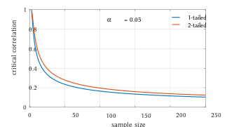
Critical values of Pearson’s correlation coefficient that must be exceeded to be considered significantly nonzero at the 0.05 level.
For pairs from an uncorrelated bivariate normal distribution, the sampling distribution of the studentized Pearson’s correlation coefficient follows Student’s t-distribution with degrees of freedom n − 2. Specifically, if the underlying variables have a bivariate normal distribution, the variable
has a student’s t-distribution in the null case (zero correlation).[23] This holds approximately in case of non-normal observed values if sample sizes are large enough.[24] For determining the critical values for r the inverse function is needed:
Alternatively, large sample, asymptotic approaches can be used.
Another early paper[25] provides graphs and tables for general values of ρ, for small sample sizes, and discusses computational approaches.
In the case where the underlying variables are not normal, the sampling distribution of Pearson’s correlation coefficient follows a Student’s t-distribution, but the degrees of freedom are reduced.[26]
Using the exact distribution[edit]
For data that follow a bivariate normal distribution, the exact density function f(r) for the sample correlation coefficient r of a normal bivariate is[27][28][29]
where is the gamma function and is the Gaussian hypergeometric function.
In the special case when (zero population correlation), the exact density function f(r) can be written as:
where is the beta function, which is one way of writing the density of a Student’s t-distribution, as above.
Using the exact confidence distribution[edit]
Confidence intervals and tests can be calculated from a confidence distribution. An exact confidence density for ρ is[30]
where is the Gaussian hypergeometric function and .
Using the Fisher transformation[edit]
In practice, confidence intervals and hypothesis tests relating to ρ are usually carried out using the Fisher transformation, :
F(r) approximately follows a normal distribution with
- and standard error
where n is the sample size. The approximation error is lowest for a large sample size and small and and increases otherwise.
Using the approximation, a z-score is
under the null hypothesis that , given the assumption that the sample pairs are independent and identically distributed and follow a bivariate normal distribution. Thus an approximate p-value can be obtained from a normal probability table. For example, if z = 2.2 is observed and a two-sided p-value is desired to test the null hypothesis that , the p-value is 2 Φ(−2.2) = 0.028, where Φ is the standard normal cumulative distribution function.
To obtain a confidence interval for ρ, we first compute a confidence interval for F():
The inverse Fisher transformation brings the interval back to the correlation scale.
For example, suppose we observe r = 0.7 with a sample size of n=50, and we wish to obtain a 95% confidence interval for ρ. The transformed value is arctanh(r) = 0.8673, so the confidence interval on the transformed scale is 0.8673 ± 1.96/√47, or (0.5814, 1.1532). Converting back to the correlation scale yields (0.5237, 0.8188).
In least squares regression analysis[edit]
The square of the sample correlation coefficient is typically denoted r2 and is a special case of the coefficient of determination. In this case, it estimates the fraction of the variance in Y that is explained by X in a simple linear regression. So if we have the observed dataset and the fitted dataset then as a starting point the total variation in the Yi around their average value can be decomposed as follows
where the are the fitted values from the regression analysis. This can be rearranged to give
The two summands above are the fraction of variance in Y that is explained by X (right) and that is unexplained by X (left).
Next, we apply a property of least square regression models, that the sample covariance between and is zero. Thus, the sample correlation coefficient between the observed and fitted response values in the regression can be written (calculation is under expectation, assumes Gaussian statistics)
Thus
where is the proportion of variance in Y explained by a linear function of X.
In the derivation above, the fact that
can be proved by noticing that the partial derivatives of the residual sum of squares (RSS) over β0 and β1 are equal to 0 in the least squares model, where
- .
In the end, the equation can be written as:
where
The symbol is called the regression sum of squares, also called the explained sum of squares, and is the total sum of squares (proportional to the variance of the data).
Sensitivity to the data distribution[edit]
Existence[edit]
The population Pearson correlation coefficient is defined in terms of moments, and therefore exists for any bivariate probability distribution for which the population covariance is defined and the marginal population variances are defined and are non-zero. Some probability distributions, such as the Cauchy distribution, have undefined variance and hence ρ is not defined if X or Y follows such a distribution. In some practical applications, such as those involving data suspected to follow a heavy-tailed distribution, this is an important consideration. However, the existence of the correlation coefficient is usually not a concern; for instance, if the range of the distribution is bounded, ρ is always defined.
Sample size[edit]
- If the sample size is moderate or large and the population is normal, then, in the case of the bivariate normal distribution, the sample correlation coefficient is the maximum likelihood estimate of the population correlation coefficient, and is asymptotically unbiased and efficient, which roughly means that it is impossible to construct a more accurate estimate than the sample correlation coefficient.
- If the sample size is large and the population is not normal, then the sample correlation coefficient remains approximately unbiased, but may not be efficient.
- If the sample size is large, then the sample correlation coefficient is a consistent estimator of the population correlation coefficient as long as the sample means, variances, and covariance are consistent (which is guaranteed when the law of large numbers can be applied).
- If the sample size is small, then the sample correlation coefficient r is not an unbiased estimate of ρ.[10] The adjusted correlation coefficient must be used instead: see elsewhere in this article for the definition.
- Correlations can be different for imbalanced dichotomous data when there is variance error in sample.[31]
Robustness[edit]
Like many commonly used statistics, the sample statistic r is not robust,[32] so its value can be misleading if outliers are present.[33][34] Specifically, the PMCC is neither distributionally robust,[citation needed] nor outlier resistant[32] (see Robust statistics § Definition). Inspection of the scatterplot between X and Y will typically reveal a situation where lack of robustness might be an issue, and in such cases it may be advisable to use a robust measure of association. Note however that while most robust estimators of association measure statistical dependence in some way, they are generally not interpretable on the same scale as the Pearson correlation coefficient.
Statistical inference for Pearson’s correlation coefficient is sensitive to the data distribution. Exact tests, and asymptotic tests based on the Fisher transformation can be applied if the data are approximately normally distributed, but may be misleading otherwise. In some situations, the bootstrap can be applied to construct confidence intervals, and permutation tests can be applied to carry out hypothesis tests. These non-parametric approaches may give more meaningful results in some situations where bivariate normality does not hold. However the standard versions of these approaches rely on exchangeability of the data, meaning that there is no ordering or grouping of the data pairs being analyzed that might affect the behavior of the correlation estimate.
A stratified analysis is one way to either accommodate a lack of bivariate normality, or to isolate the correlation resulting from one factor while controlling for another. If W represents cluster membership or another factor that it is desirable to control, we can stratify the data based on the value of W, then calculate a correlation coefficient within each stratum. The stratum-level estimates can then be combined to estimate the overall correlation while controlling for W.[35]
Variants[edit]
Variations of the correlation coefficient can be calculated for different purposes. Here are some examples.
Adjusted correlation coefficient[edit]
The sample correlation coefficient r is not an unbiased estimate of ρ. For data that follows a bivariate normal distribution, the expectation E[r] for the sample correlation coefficient r of a normal bivariate is[36]
- therefore r is a biased estimator of
The unique minimum variance unbiased estimator radj is given by[37]
-
(1)
where:
An approximately unbiased estimator radj can be obtained[citation needed] by truncating E[r] and solving this truncated equation:
-
(2)
An approximate solution[citation needed] to equation (2) is:
-
(3)
where in (3):
- are defined as above,
- radj is a suboptimal estimator,[citation needed][clarification needed]
- radj can also be obtained by maximizing log(f(r)),
- radj has minimum variance for large values of n,
- radj has a bias of order 1⁄(n − 1).
Another proposed[10] adjusted correlation coefficient is:[citation needed]
Note that radj ≈ r for large values of n.
Weighted correlation coefficient[edit]
Suppose observations to be correlated have differing degrees of importance that can be expressed with a weight vector w. To calculate the correlation between vectors x and y with the weight vector w (all of length n),[38][39]
- Weighted mean:
- Weighted covariance
- Weighted correlation
Reflective correlation coefficient[edit]
The reflective correlation is a variant of Pearson’s correlation in which the data are not centered around their mean values.[citation needed] The population reflective correlation is
The reflective correlation is symmetric, but it is not invariant under translation:
The sample reflective correlation is equivalent to cosine similarity:
The weighted version of the sample reflective correlation is
Scaled correlation coefficient[edit]
Scaled correlation is a variant of Pearson’s correlation in which the range of the data is restricted intentionally and in a controlled manner to reveal correlations between fast components in time series.[40] Scaled correlation is defined as average correlation across short segments of data.
Let be the number of segments that can fit into the total length of the signal for a given scale :
The scaled correlation across the entire signals is then computed as
where is Pearson’s coefficient of correlation for segment .
By choosing the parameter , the range of values is reduced and the correlations on long time scale are filtered out, only the correlations on short time scales being revealed. Thus, the contributions of slow components are removed and those of fast components are retained.
Pearson’s distance[edit]
A distance metric for two variables X and Y known as Pearson’s distance can be defined from their correlation coefficient as[41]
Considering that the Pearson correlation coefficient falls between [−1, +1], the Pearson distance lies in [0, 2]. The Pearson distance has been used in cluster analysis and data detection for communications and storage with unknown gain and offset.[42]
The Pearson «distance» defined this way assigns distance greater than 1 to negative correlations. In reality, both strong positive correlation and negative correlations are meaningful, so care must be taken when Pearson «distance» is used for nearest neighbor algorithm as such algorithm will only include neighbors with positive correlation and exclude neighbors with negative correlation. Alternatively, an absolute valued distance: can be applied, which will take both positive and negative correlations into consideration. The information on positive and negative association can be extracted separately, later.
Circular correlation coefficient[edit]
For variables X = {x1,…,xn} and Y = {y1,…,yn} that are defined on the unit circle [0, 2π), it is possible to define a circular analog of Pearson’s coefficient.[43] This is done by transforming data points in X and Y with a sine function such that the correlation coefficient is given as:
where and are the circular means of X and Y. This measure can be useful in fields like meteorology where the angular direction of data is important.
Partial correlation[edit]
If a population or data-set is characterized by more than two variables, a partial correlation coefficient measures the strength of dependence between a pair of variables that is not accounted for by the way in which they both change in response to variations in a selected subset of the other variables.
Decorrelation of n random variables[edit]
It is always possible to remove the correlations between all pairs of an arbitrary number of random variables by using a data transformation, even if the relationship between the variables is nonlinear. A presentation of this result for population distributions is given by Cox & Hinkley.[44]
A corresponding result exists for reducing the sample correlations to zero. Suppose a vector of n random variables is observed m times. Let X be a matrix where is the jth variable of observation i. Let be an m by m square matrix with every element 1. Then D is the data transformed so every random variable has zero mean, and T is the data transformed so all variables have zero mean and zero correlation with all other variables – the sample correlation matrix of T will be the identity matrix. This has to be further divided by the standard deviation to get unit variance. The transformed variables will be uncorrelated, even though they may not be independent.
where an exponent of −+1⁄2 represents the matrix square root of the inverse of a matrix. The correlation matrix of T will be the identity matrix. If a new data observation x is a row vector of n elements, then the same transform can be applied to x to get the transformed vectors d and t:
This decorrelation is related to principal components analysis for multivariate data.
Software implementations[edit]
- R’s statistics base-package implements the correlation coefficient with
cor(x, y), or (with the P value also) withcor.test(x, y). - The SciPy Python library via
pearsonr(x, y). - The Pandas Python library implements Pearson correlation coefficient calculation as the default option for the method
pandas.DataFrame.corr - Wolfram Mathematica via the
Correlationfunction, or (with the P value) withCorrelationTest. - The Boost C++ library via the
correlation_coefficientfunction. - Excel has an in-built
correl(array1, array2)function for calculationg the pearson’s correlation coefficient.
See also[edit]
- Anscombe’s quartet
- Association (statistics)
- Coefficient of colligation
- Yule’s Q
- Yule’s Y
- Concordance correlation coefficient
- Correlation and dependence
- Correlation ratio
- Disattenuation
- Distance correlation
- Maximal information coefficient
- Multiple correlation
- Normally distributed and uncorrelated does not imply independent
- Odds ratio
- Partial correlation
- Polychoric correlation
- Quadrant count ratio
- RV coefficient
- Spearman’s rank correlation coefficient
Footnotes[edit]
- ^ As early as 1877, Galton was using the term «reversion» and the symbol «r» for what would become «regression».[3][4][5]
References[edit]
- ^ «SPSS Tutorials: Pearson Correlation».
- ^ «Correlation Coefficient: Simple Definition, Formula, Easy Steps». Statistics How To.
- ^ Galton, F. (5–19 April 1877). «Typical laws of heredity». Nature. 15 (388, 389, 390): 492–495, 512–514, 532–533. Bibcode:1877Natur..15..492.. doi:10.1038/015492a0. S2CID 4136393. In the «Appendix» on page 532, Galton uses the term «reversion» and the symbol r.
- ^ Galton, F. (24 September 1885). «The British Association: Section II, Anthropology: Opening address by Francis Galton, F.R.S., etc., President of the Anthropological Institute, President of the Section». Nature. 32 (830): 507–510.
- ^ Galton, F. (1886). «Regression towards mediocrity in hereditary stature». Journal of the Anthropological Institute of Great Britain and Ireland. 15: 246–263. doi:10.2307/2841583. JSTOR 2841583.
- ^ Pearson, Karl (20 June 1895). «Notes on regression and inheritance in the case of two parents». Proceedings of the Royal Society of London. 58: 240–242. Bibcode:1895RSPS…58..240P.
- ^ Stigler, Stephen M. (1989). «Francis Galton’s account of the invention of correlation». Statistical Science. 4 (2): 73–79. doi:10.1214/ss/1177012580. JSTOR 2245329.
- ^ «Analyse mathematique sur les probabilités des erreurs de situation d’un point». Mem. Acad. Roy. Sci. Inst. France. Sci. Math, et Phys. (in French). 9: 255–332. 1844 – via Google Books.
- ^ Wright, S. (1921). «Correlation and causation». Journal of Agricultural Research. 20 (7): 557–585.
- ^ a b c d e Real Statistics Using Excel: Correlation: Basic Concepts, retrieved 22 February 2015
- ^ Weisstein, Eric W. «Statistical Correlation». mathworld.wolfram.com. Retrieved 22 August 2020.
- ^ Moriya, N. (2008). «Noise-related multivariate optimal joint-analysis in longitudinal stochastic processes». In Yang, Fengshan (ed.). Progress in Applied Mathematical Modeling. Nova Science Publishers, Inc. pp. 223–260. ISBN 978-1-60021-976-4.
- ^ Garren, Steven T. (15 June 1998). «Maximum likelihood estimation of the correlation coefficient in a bivariate normal model, with missing data». Statistics & Probability Letters. 38 (3): 281–288. doi:10.1016/S0167-7152(98)00035-2.
- ^ «2.6 — (Pearson) Correlation Coefficient r». STAT 462. Retrieved 10 July 2021.
- ^ «Introductory Business Statistics: The Correlation Coefficient r». opentextbc.ca. Retrieved 21 August 2020.
- ^ Rodgers; Nicewander (1988). «Thirteen ways to look at the correlation coefficient» (PDF). The American Statistician. 42 (1): 59–66. doi:10.2307/2685263. JSTOR 2685263.
- ^ Schmid, John Jr. (December 1947). «The relationship between the coefficient of correlation and the angle included between regression lines». The Journal of Educational Research. 41 (4): 311–313. doi:10.1080/00220671.1947.10881608. JSTOR 27528906.
- ^ Rummel, R.J. (1976). «Understanding Correlation». ch. 5 (as illustrated for a special case in the next paragraph).
- ^ Buda, Andrzej; Jarynowski, Andrzej (December 2010). Life Time of Correlations and its Applications. Wydawnictwo Niezależne. pp. 5–21. ISBN 9788391527290.
- ^ a b Cohen, J. (1988). Statistical Power Analysis for the Behavioral Sciences (2nd ed.).
- ^ Bowley, A. L. (1928). «The Standard Deviation of the Correlation Coefficient». Journal of the American Statistical Association. 23 (161): 31–34. doi:10.2307/2277400. ISSN 0162-1459. JSTOR 2277400.
- ^ «Derivation of the standard error for Pearson’s correlation coefficient». Cross Validated. Retrieved 30 July 2021.
- ^ Rahman, N. A. (1968) A Course in Theoretical Statistics, Charles Griffin and Company, 1968
- ^ Kendall, M. G., Stuart, A. (1973) The Advanced Theory of Statistics, Volume 2: Inference and Relationship, Griffin. ISBN 0-85264-215-6 (Section 31.19)
- ^ Soper, H.E.; Young, A.W.; Cave, B.M.; Lee, A.; Pearson, K. (1917). «On the distribution of the correlation coefficient in small samples. Appendix II to the papers of «Student» and R.A. Fisher. A co-operative study». Biometrika. 11 (4): 328–413. doi:10.1093/biomet/11.4.328.
- ^ Davey, Catherine E.; Grayden, David B.; Egan, Gary F.; Johnston, Leigh A. (January 2013). «Filtering induces correlation in fMRI resting state data». NeuroImage. 64: 728–740. doi:10.1016/j.neuroimage.2012.08.022. hdl:11343/44035. PMID 22939874. S2CID 207184701.
- ^ Hotelling, Harold (1953). «New Light on the Correlation Coefficient and its Transforms». Journal of the Royal Statistical Society. Series B (Methodological). 15 (2): 193–232. doi:10.1111/j.2517-6161.1953.tb00135.x. JSTOR 2983768.
- ^ Kenney, J.F.; Keeping, E.S. (1951). Mathematics of Statistics. Vol. Part 2 (2nd ed.). Princeton, NJ: Van Nostrand.
- ^ Weisstein, Eric W. «Correlation Coefficient—Bivariate Normal Distribution». mathworld.wolfram.com.
- ^ Taraldsen, Gunnar (2020). «Confidence in Correlation». doi:10.13140/RG.2.2.23673.49769.
- ^ Lai, Chun Sing; Tao, Yingshan; Xu, Fangyuan; Ng, Wing W.Y.; Jia, Youwei; Yuan, Haoliang; Huang, Chao; Lai, Loi Lei; Xu, Zhao; Locatelli, Giorgio (January 2019). «A robust correlation analysis framework for imbalanced and dichotomous data with uncertainty» (PDF). Information Sciences. 470: 58–77. doi:10.1016/j.ins.2018.08.017. S2CID 52878443.
- ^ a b Wilcox, Rand R. (2005). Introduction to robust estimation and hypothesis testing. Academic Press.
- ^ Devlin, Susan J.; Gnanadesikan, R.; Kettenring J.R. (1975). «Robust estimation and outlier detection with correlation coefficients». Biometrika. 62 (3): 531–545. doi:10.1093/biomet/62.3.531. JSTOR 2335508.
- ^ Huber, Peter. J. (2004). Robust Statistics. Wiley.[page needed]
- ^ Katz., Mitchell H. (2006) Multivariable Analysis – A Practical Guide for Clinicians. 2nd Edition. Cambridge University Press. ISBN 978-0-521-54985-1. ISBN 0-521-54985-X
- ^ Hotelling, H. (1953). «New Light on the Correlation Coefficient and its Transforms». Journal of the Royal Statistical Society. Series B (Methodological). 15 (2): 193–232. doi:10.1111/j.2517-6161.1953.tb00135.x. JSTOR 2983768.
- ^ Olkin, Ingram; Pratt,John W. (March 1958). «Unbiased Estimation of Certain Correlation Coefficients». The Annals of Mathematical Statistics. 29 (1): 201–211. doi:10.1214/aoms/1177706717. JSTOR 2237306..
- ^ «Re: Compute a weighted correlation». sci.tech-archive.net.
- ^ «Weighted Correlation Matrix – File Exchange – MATLAB Central».
- ^ Nikolić, D; Muresan, RC; Feng, W; Singer, W (2012). «Scaled correlation analysis: a better way to compute a cross-correlogram» (PDF). European Journal of Neuroscience. 35 (5): 1–21. doi:10.1111/j.1460-9568.2011.07987.x. PMID 22324876. S2CID 4694570.
- ^ Fulekar (Ed.), M.H. (2009) Bioinformatics: Applications in Life and Environmental Sciences, Springer (pp. 110) ISBN 1-4020-8879-5
- ^ Immink, K. Schouhamer; Weber, J. (October 2010). «Minimum Pearson distance detection for multilevel channels with gain and / or offset mismatch». IEEE Transactions on Information Theory. 60 (10): 5966–5974. CiteSeerX 10.1.1.642.9971. doi:10.1109/tit.2014.2342744. S2CID 1027502. Retrieved 11 February 2018.
- ^ Jammalamadaka, S. Rao; SenGupta, A. (2001). Topics in circular statistics. New Jersey: World Scientific. p. 176. ISBN 978-981-02-3778-3. Retrieved 21 September 2016.
- ^ Cox, D.R.; Hinkley, D.V. (1974). Theoretical Statistics. Chapman & Hall. Appendix 3. ISBN 0-412-12420-3.
External links[edit]
- «cocor». comparingcorrelations.org. – A free web interface and R package for the statistical comparison of two dependent or independent correlations with overlapping or non-overlapping variables.
- «Correlation». nagysandor.eu. – an interactive Flash simulation on the correlation of two normally distributed variables.
- «Correlation coefficient calculator». hackmath.net. Linear regression. –
- «Critical values for Pearson’s correlation coefficient» (PDF). frank.mtsu.edu/~dkfuller. – large table.
- «Guess the Correlation». – A game where players guess how correlated two variables in a scatter plot are, in order to gain a better understanding of the concept of correlation.
Чем больше я узнаю людей, тем больше мне нравится моя собака.
—Марк Твен
В предыдущих сериях постов для начинающих из ремикса книги Генри Гарнера «Clojure для исследования данных» (Clojure for Data Science) на языке Python мы рассмотрели методы описания выборок с точки зрения сводных статистик и методов статистического вывода из них параметров популяции. Такой анализ сообщает нам нечто о популяции в целом и о выборке в частности, но он не позволяет нам делать очень точные утверждения об их отдельных элементах. Это связано с тем, что в результате сведения данных всего к двум статистикам — среднему значению и стандартному отклонению — теряется огромный объем информации.
Нам часто требуется пойти дальше и установить связь между двумя или несколькими переменными либо предсказать одну переменную при наличии другой. И это подводит нас к теме данной серии из 5 постов — исследованию корреляции и регрессии. Корреляция имеет дело с силой и направленностью связи между двумя или более переменными. Регрессия определяет природу этой связи и позволяет делать предсказания на ее основе.
В этой серии постов будет рассмотрена линейная регрессия. При наличии выборки данных наша модель усвоит линейное уравнение, позволяющее ей делать предсказания о новых, не встречавшихся ранее данных. Для этого мы снова обратимся к библиотеке pandas и изучим связь между ростом и весом спортсменов-олимпийцев. Мы введем понятие матриц и покажем способы управления ими с использованием библиотеки pandas.
О данных
В этой серии постов используются данные, любезно предоставленные компанией Guardian News and Media Ltd., о спортсменах, принимавших участие в Олимпийских Играх 2012 г. в Лондоне. Эти данные изначально были взяты из блога газеты Гардиан.
Обследование данных
Когда вы сталкиваетесь с новым набором данных, первая задача состоит в том, чтобы его обследовать с целью понять, что именно он содержит.
Файл all-london-2012-athletes.tsv достаточно небольшой. Мы можем обследовать данные при помощи pandas, как мы делали в первой серии постов «Python, исследование данных и выборы», воспользовавшись функцией read_csv:
def load_data():
    return pd.read_csv('data/ch03/all-london-2012-athletes-ru.tsv', 't')

def ex_3_1():
    '''Загрузка данных об участниках
       олимпийских игр в Лондоне 2012 г.'''
    return load_data()
Если выполнить этот пример в консоли интерпретатора Python либо в блокноте Jupyter, то вы должны увидеть следующий ниже результат:

Столбцы данных (нам повезло, что они ясно озаглавлены) содержат следующую информацию:
-
ФИО атлета
-
страна, за которую он выступает
-
возраст, лет
-
рост, см.
-
вес, кг.
-
пол «М» или «Ж»
-
дата рождения в виде строки
-
место рождения в виде строки (со страной)
-
число выигранных золотых медалей
-
число выигранных серебряных медалей
-
число выигранных бронзовых медалей
-
всего выигранных золотых, серебряных и бронзовых медалей
-
вид спорта, в котором он соревновался
-
состязание в виде списка, разделенного запятыми
Даже с учетом того, что данные четко озаглавлены, очевидно присутствие пустых мест в столбцах с ростом, весом и местом рождения. При наличии таких данных следует проявлять осторожность, чтобы они не сбили с толку.
Визуализация данных
В первую очередь мы рассмотрим разброс роста спортсменов на Олимпийских играх 2012 г. в Лондоне. Изобразим эти значения роста в виде гистограммы, чтобы увидеть характер распределения данных, не забыв сначала отфильтровать пропущенные значения:
def ex_3_2():
    '''Визуализация разброса значений
       роста спортсменов на гистограмме'''
    df = load_data()
    df['Рост, см'].hist(bins=20)
    plt.xlabel('Рост, см.')
    plt.ylabel('Частота')
    plt.show()
Этот пример сгенерирует следующую ниже гистограмму:
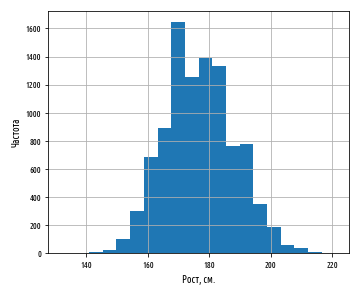
Как мы и ожидали, данные приближенно нормально распределены. Средний рост спортсменов составляет примерно 177 см. Теперь посмотрим на распределение веса олимпийских спортсменов:
def ex_3_3():
    '''Визуализация разброса значений веса спортсменов'''
    df = load_data()
    df['Вес'].hist(bins=20)
    plt.xlabel('Вес')
    plt.ylabel('Частота')
    plt.show()
Приведенный выше пример сгенерирует следующую ниже гистограмму:
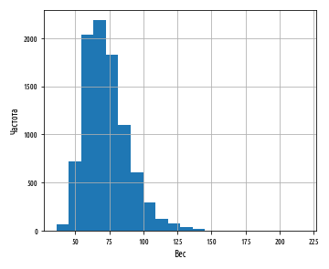
Данные показывают четко выраженную асимметрию. Хвост с правой стороны намного длиннее, чем с левой, и поэтому мы говорим, что асимметрия — положительная. Мы можем оценить асимметрию данных количественно при помощи функции библиотеки pandas skew:
def ex_3_4():
    '''Вычисление асимметрии веса спортсменов'''
    df = load_data()
    swimmers = df[ df['Вид спорта'] == 'Swimming']
return swimmers['Вес'].skew()0.23441459903001483К счастью, эта асимметрия может быть эффективным образом смягчена путем взятия логарифма веса при помощи функции библиотеки numpy np.log:
def ex_3_5():
    '''Визуализация разброса значений веса спортсменов на
       полулогарифмической гистограмме с целью удаления
       асимметрии'''
    df = load_data()
    df['Вес'].apply(np.log).hist(bins=20)
    plt.xlabel('Логарифмический вес')
    plt.ylabel('Частота')
    plt.show()
Этот пример сгенерирует следующую ниже гистограмму:
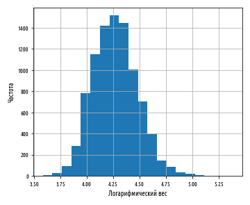
Теперь данные намного ближе к нормальному распределению. Из этого следует, что вес распределяется согласно логнормальному распределению.
Логнормальное распределение
Логнормальное распределение — это распределение набора значений, чей логарифм нормально распределен. Основание логарифма может быть любым положительным числом за исключением единицы. Как и нормальное распределение, логнормальное распределение играет важную роль для описания многих естественных явлений.
Логарифм показывает степень, в которую должно быть возведено фиксированное число (основание) для получения данного числа. Изобразив логарифмы на графике в виде гистограммы, мы показали, что эти степени приближенно нормально распределены. Логарифмы обычно берутся по основанию 10 или основанию e, трансцендентному числу, приближенно равному 2.718. В функции библиотеки numpy np.log и ее инверсии np.exp используется основание e. Выражение loge также называется натуральным логарифмом, или ln, из-за свойств, делающих его особенно удобным в исчислении.
Логнормальное распределение обычно имеет место в процессах роста, где темп роста не зависит от размера. Этот феномен известен как закон Джибрэта, который был cформулирован в 1931 г. Робертом Джибрэтом, заметившим, что он применим к росту фирм. Поскольку темп роста пропорционален размеру, более крупные фирмы демонстрируют тенденцию расти быстрее, чем фирмы меньшего размера.
Нормальное распределение случается в ситуациях, где много мелких колебаний, или вариаций, носит суммирующий эффект, тогда как логнормальное распределение происходит там, где много мелких вариаций имеет мультипликативный эффект.
С тех пор выяснилось, что закон Джибрэта применим к большому числу ситуаций, включая размеры городов и, согласно обширному математическому ресурсу Wolfram MathWorld, к количеству слов в предложениях шотландского писателя Джорджа Бернарда Шоу.
В остальной части этой серии постов мы будем использовать натуральный логарифм веса спортсменов, чтобы наши данные были приближенно нормально распределены. Мы выберем популяцию спортсменов примерно с одинаковыми типами телосложения, к примеру, олимпийских пловцов.
Визуализация корреляции
Один из самых быстрых и самых простых способов определить наличие корреляции между двумя переменными состоит в том, чтобы рассмотреть их на графике рассеяния. Мы отфильтруем данные, выбрав только пловцов, и затем построим график роста относительно веса спортсменов:
def swimmer_data():
    '''Загрузка данных роста и веса только олимпийских пловцов'''
    df = load_data()
    return df[df['Вид спорта'] == 'Swimming'].dropna()

def ex_3_6():
    '''Визуализация корреляции между ростом и весом'''
    df = swimmer_data()
    xs = df['Рост, см']
    ys = df['Вес'].apply( np.log )
    pd.DataFrame(np.array([xs,ys]).T).plot.scatter(0, 1, s=12, grid=True)
    plt.xlabel('Рост, см.')
    plt.ylabel('Логарифмический вес')
    plt.show()
Этот пример сгенерирует следующий ниже график:
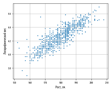
Результат ясно показывает, что между этими двумя переменными имеется связь. График имеет характерно смещенную эллиптическую форму двух коррелируемых, нормально распределенных переменных с центром вокруг среднего значения. Следующая ниже диаграмма сравнивает график рассеяния с распределениями вероятностей роста и логарифма веса:
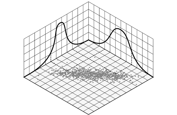
Точки, близко расположенные к хвосту одного распределения, также демонстрируют тенденцию близко располагаться к тому же хвосту другого распределения, и наоборот. Таким образом, между двумя распределениями существует связь, которую в ближайших нескольких разделах мы покажем, как определять количественно. Впрочем, если мы внимательно посмотрим на предыдущий график рассеяния, то увидим, что из-за округления измерений точки уложены в столбцы и строки (в см. и кг. соответственно для роста и веса). Там, где это происходит, иногда желательно внести в данные искажения, которые также называются сдвигом или джиттером с тем, чтобы яснее показать силу связи. Без генерирования джиттера (в виде случайных отклонений) может оказаться, что, то, что по внешнему виду составляет одну точку, фактически представляет много точек, которые обозначены одинаковой парой значений. Внесение нескольких случайных помех делает эту ситуацию вряд ли возможной.
Генерирование джиттера
Поскольку каждое значение округлено до ближайшего сантиметра или килограмма, то значение, записанное как 180 см, на самом деле может быть каким угодно между 179.5 и 180.5 см, тогда как значение 80 кг на самом деле может быть каким угодно между 79.5 и 80.5 кг. Для создания случайных искажений, мы можем добавить случайные помехи в каждую точку данных роста в диапазоне между -0.5 и 0.5 и в том же самом диапазоне проделать с точками данных веса (разумеется, это нужно cделать до того, как мы возьмем логарифм значений веса):
def jitter(limit):
    '''Генератор джиттера (произвольного сдвига точек данных)'''
    return lambda x: random.uniform(-limit, limit) + x

def ex_3_7():
    '''Визуализация корреляции между ростом и весом с джиттером'''
    df = swimmer_data()
    xs = df['Рост, см'].apply(jitter(0.5))
    ys = df['Вес'].apply(jitter(0.5)).apply(np.log)
    pd.DataFrame(np.array([xs,ys]).T).plot.scatter(0, 1, s=12, grid=True)
    plt.xlabel('Рост, см.')
    plt.ylabel('Логарифмический вес')
    plt.show()
График с джиттером выглядит следующим образом:
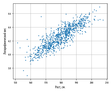
Как и в случае с внесением прозрачности в график рассеяния в первой серии постов об описательной статистике, генерирование джиттера — это механизм, который обеспечивает исключение несущественных факторов, таких как объем данных или артефакты округления, которые могут заслонить от нас возможность увидеть закономерности в данных.
Ковариация
Одним из способов количественного определения силы связи между двумя переменными является их ковариация. Она измеряет тенденцию двух переменных изменяться вместе.
Если у нас имеется два ряда чисел, X и Y, то их отклонения от среднего значения составляют:
![]()
![]()
Здесь xi — это значение X с индексом i, yi — значение Y с индексом i, x̅ — среднее значение X, и y̅ — среднее значение Y. Если X и Y проявляют тенденцию изменяться вместе, то их отклонения от среднего будет иметь одинаковый знак: отрицательный, если они — меньше среднего, положительный, если они больше среднего. Если мы их перемножим, то произведение будет положительным, когда у них одинаковый знак, и отрицательным, когда у них разные знаки. Сложение произведений дает меру тенденции этих двух переменных отклоняться от среднего значения в одинаковом направлении для каждой заданной выборки.
Ковариация определяется как среднее этих произведений:
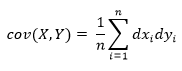
На чистом Python ковариация вычисляется следующим образом:
def covariance(xs, ys):
    '''Вычисление ковариации (несмещенная, т.е. n-1)'''
    dx = xs - xs.mean()
    dy = ys - ys.mean()
    return (dx * dy).sum() / (dx.count() - 1)
В качестве альтернативы, мы можем воспользоваться функцией pandas cov:
df['Рост, см'].cov(df['Вес'])1.3559273321696459Ковариация роста и логарифма веса для наших олимпийских пловцов равна 1.356, однако это число сложно интерпретировать. Единицы измерения здесь представлены произведением единиц на входе.
По этой причине о ковариации редко сообщают как об отдельной сводной статистике. Сделать число более понятным можно, разделив отклонения на произведение стандартных отклонений. Это позволяет трансформировать единицы измерения в стандартные оценки и ограничить выход числом в диапазоне между -1 и +1. Этот результат называется корреляцией Пирсона.
Стандартная оценка, англ. standard score, также z-оценка — это относительное число стандартных отклонений, на которые значение переменной отстоит от среднего значения. Положительная оценка показывает, что переменная находится выше среднего, отрицательная — ниже среднего. Это безразмерная величина, получаемая при вычитании популяционного среднего из индивидуальных значений и деления разности на популяционное стандартное отклонение.
Корреляция Пирсона
Корреляция Пирсона часто обозначается переменной r и вычисляется следующим образом, где отклонения от среднего dxi и dyi вычисляются как и прежде:
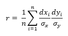
Поскольку для переменных X и Y стандартные отклонения являются константными, уравнение может быть упрощено до следующего, где σx и σy — это стандартные отклонения соответственно X и Y:
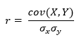
В таком виде формула иногда упоминается как коэффициент корреляции смешанных моментов Пирсона или попросту коэффициент корреляции и, как правило, обозначается буквой r.
Ранее мы уже написали функции для вычисления стандартного отклонения. В сочетании с нашей функцией с вычислением ковариации получится следующая ниже имплементация корреляции Пирсона:
def variance(xs):
    '''Вычисление корреляции,
       несмещенная дисперсия при n <= 30'''
    x_hat = xs.mean()
    n = xs.count()
    n = n - 1 if n in range( 1, 30 ) else n
    return sum((xs - x_hat) ** 2) / n

def standard_deviation(xs):
    '''Вычисление стандартного отклонения'''
    return np.sqrt(variance(xs))

def correlation(xs, ys):
    '''Вычисление корреляции'''
    return covariance(xs, ys) / (standard_deviation(xs) *
                                 standard_deviation(ys))
В качестве альтернативы мы можем воспользоваться функцией pandas corr:
df['Рост, см'].corr(df['Вес'])Поскольку стандартные оценки безразмерны, то и коэффициент корреляции r тоже безразмерен. Если r равен -1.0 либо 1.0, то переменные идеально антикоррелируют либо идеально коррелируют.
Правда, если r = 0, то с необходимостью вовсе не следует, что переменные не коррелируют. Корреляция Пирсона измеряет лишь линейные связи. Как продемонстрировано на следующих графиках, между переменными может существовать еще некая нелинейная связь, которую r не объясняет:
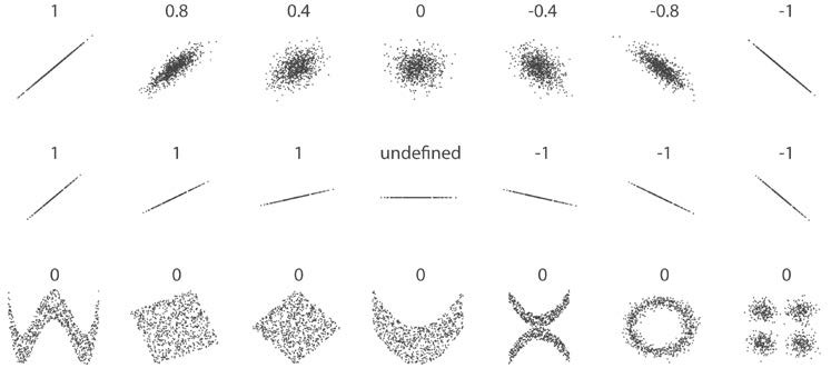
Отметим, что корреляция центрального примера не определена, потому что стандартное отклонение y = 0. Поскольку наше уравнение для r содержало бы деление ковариации на 0, то результат получается бессмысленным. В этом случае между переменными не может быть никакой корреляции; y всегда будет иметь среднее значение. Простое обследование стандартных отклонений это подтвердит.
Мы можем вычислить коэффициент корреляции для данных роста и логарифма веса наших пловцов следующим образом:
def ex_3_8():
    '''Вычисление корреляции средствами pandas
       на примере данных роста и веса'''
    df = swimmer_data()
return df['Рост, см'].corr( df['Вес'].apply(np.log))0.86748249283924894В результате получим ответ 0.867, который количественно выражает сильную, положительную корреляцию, уже наблюдавшуюся нами на точечном графике.
Выборочный r и популяционный ρ
Аналогично среднему значению и стандартному отклонению, коэффициент корреляции является сводной статистикой. Он описывает выборку; в данном случае, выборку спаренных значений: роста и веса. Коэффициент корреляции известной выборки обозначается буквой r, тогда как коэффициент корреляции неизвестной популяции обозначается греческой буквой ρ (рхо).
Как мы убедились в предыдущей серии постов о тестировании гипотез, мы не должны исходить из того, что результаты, полученные в ходе измерения нашей выборки, применимы к популяции в целом. К примеру, наша популяция может состоять из всех пловцов всех недавних Олимпийских игр. И будет совершенно недопустимо обобщать, например, на другие олимпийские виды спорта, такие как тяжелая атлетика или фитнес-плавание.
Даже в допустимой популяции — такой как пловцы, выступавшие на недавних Олимпийских играх, — наша выборка коэффициента корреляции является всего лишь одной из многих потенциально возможных. То, насколько мы можем доверять нашему r, как оценке параметра ρ, зависит от двух факторов:
-
Размера выборки
-
Величины r
Безусловно, чем больше выборка, тем больше мы ей доверяем в том, что она представляет всю совокупность в целом. Возможно, не совсем интуитивно очевидно, но величина тоже оказывает влияние на степень нашей уверенности в том, что выборка представляет параметр . Это вызвано тем, что большие коэффициенты вряд ли возникли случайным образом или вследствие случайной ошибки при отборе.
Проверка статистических гипотез
В предыдущей серии постов мы познакомились с проверкой статистических гипотез, как средством количественной оценки вероятности, что конкретная гипотеза (как, например, что две выборки взяты из одной и той же популяции) истинная. Чтобы количественно оценить вероятность, что корреляция существует в более широкой популяции, мы воспользуемся той же самой процедурой.
В первую очередь, мы должны сформулировать две гипотезы, нулевую гипотезу и альтернативную:
![]()
![]()
H0 — это гипотеза, что корреляция в популяции нулевая. Другими словами, наше консервативное представление состоит в том, что измеренная корреляция целиком вызвана случайной ошибкой при отборе.
H1 — это альтернативная возможность, что корреляция в популяции не нулевая. Отметим, что мы не определяем направление корреляции, а только что она существует. Это означает, что мы выполняем двустороннюю проверку.
Стандартная ошибка коэффициента корреляции r по выборке задается следующей формулой:
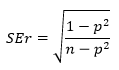
Эта формула точна, только когда r находится близко к нулю (напомним, что величина ρ влияет на нашу уверенность), но к счастью, это именно то, что мы допускаем согласно нашей нулевой гипотезы.
Мы можем снова воспользоваться t-распределением и вычислить t-статистику:
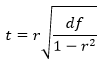
В приведенной формуле df — это степень свободы наших данных. Для проверки корреляции степень свободы равна n — 2, где n — это размер выборки. Подставив это значение в формулу, получим:
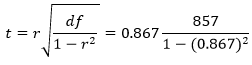
В итоге получим t-значение 102.21. В целях его преобразования в p-значение мы должны обратиться к t-распределению. Библиотека scipy предоставляет интегральную функцию распределения (ИФР) для t-распределения в виде функции stats.t.cdf, и комплементарной ей (1-cdf) функции выживания stats.t.sf. Значение функции выживания соответствует p-значению для односторонней проверки. Мы умножаем его на 2, потому что выполняем двустороннюю проверку:
def t_statistic(xs, ys):
    '''Вычисление t-статистики'''
    r = xs.corr(ys)  # как вариант, correlation(xs, ys)
    df = xs.count() - 2
    return r * np.sqrt(df / 1 - r ** 2)

def ex_3_9():
    '''Выполнение двухстороннего t-теста'''
    df = swimmer_data()
    xs = df['Рост, см']
    ys = df['Вес'].apply(np.log)
    t_value = t_statistic(xs, ys)
    df = xs.count() - 2
    p = 2 * stats.t.sf(t_value, df)  # функция выживания
    return {'t-значение':t_value, 'p-значение':p}
{'p-значение': 1.8980236317815443e-106, 't-значение': 25.384018200627057}P-значение настолько мало, что в сущности равно 0, означая, что шанс, что нулевая гипотеза является истинной, фактически не существует. Мы вынуждены принять альтернативную гипотезу о существовании корреляции.
Интервалы уверенности
Установив, что в более широкой популяции, безусловно, существует корреляция, мы, возможно, захотим количественно выразить диапазон значений, внутри которого, как мы ожидаем, будет лежать параметр ρ, вычислив для этого интервал уверенности. Как и в случае со средним значением в предыдущей серии постов, интервал уверенности для r выражает вероятность (выраженную в %), что параметр ρ популяции находится между двумя конкретными значениями.
Однако при попытке вычислить стандартную ошибку коэффициента корреляции возникает сложность, которой не было в случае со средним значением. Поскольку абсолютное значение коэффициента корреляции r не может превышать 1, распределение возможных выборок коэффициентов корреляции r смещается по мере приближения r к пределу своего диапазона.
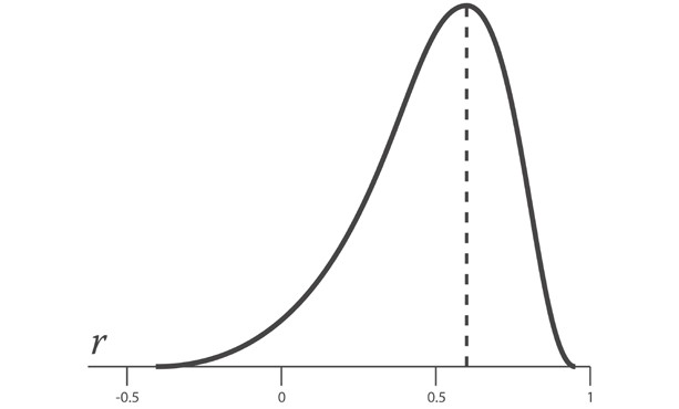
Приведенный выше график показывает отрицательно скошенное распределение r-выборок для параметра ρ, равного 0.6.
К счастью, трансформация под названием z-преобразование Фишера стабилизирует дисперсию r по своему диапазону. Она аналогична тому, как наши данные о весе спортсменов стали нормально распределенными, когда мы взяли их логарифм.
Уравнение для z-преобразования следующее:
![]()
Стандартная ошибка z равна:

Таким образом, процедура вычисления интервалов уверенности состоит в преобразовании r в z с использованием z-преобразования, вычислении интервала уверенности в терминах стандартной ошибки SEz и затем преобразовании интервала уверенности в r.
В целях вычисления интервала уверенности в терминах SEz, мы можем взять число стандартных отклонений от среднего, которое дает нам требуемый уровень доверия. Обычно используют число 1.96, так как оно является числом стандартных отклонений от среднего, которое содержит 95% площади под кривой. Другими словами, 1.96 стандартных ошибок от среднего значения выборочного r содержит истинную популяционную корреляцию ρ с 95%-ой определенностью.
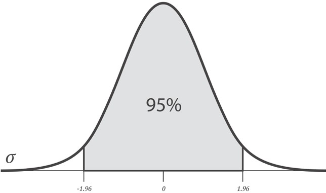
Мы можем убедиться в этом, воспользовавшись функцией scipy stats.norm.ppf. Она вернет стандартную оценку, связанную с заданной интегральной вероятностью в условиях односторонней проверки.
Однако, как показано на приведенном выше графике, мы хотели бы вычесть ту же самую величину, т.е. 2.5%, из каждого хвоста с тем, чтобы 95%-й интервал уверенности был центрирован на нуле. Для этого при выполнении двусторонней проверки нужно просто уменьшить разность наполовину и вычесть результат из 100%. Так что, требуемый уровень доверия в 95% означает, что мы обращаемся к критическому значению 97.5%:
def critical_value(confidence, ntails): # ДИ и число хвостов
    '''Расчет критического значения путем
       вычисления квантиля и получения
       для него нормального значения'''
    lookup = 1 - ((1 - confidence) / ntails)
    return stats.norm.ppf(lookup, 0, 1)  # mu=0, sigma=1

critical_value(0.95, 2)1.959963984540054Поэтому наш 95%-й интервал уверенности в z-пространстве для ρ задается следующей формулой:
![]()
Подставив в нашу формулу zr и SEz, получим:
![]()
Для r=0.867 и n=859 она даст нижнюю и верхнюю границу соответственно 1.137 и 1.722. В целях их преобразования из z-оценок в r-значения, мы используем следующее обратное уравнение z-преобразования:

Преобразования и интервал уверенности можно вычислить при помощи следующего исходного кода:
def z_to_r(z):
    '''Преобразование z-оценки обратно в r-значение'''
    return (np.exp(z*2) - 1) / (np.exp(z*2) + 1)

def r_confidence_interval(crit, xs, ys):
    '''Расчет интервала уверенности
       для критического значения и данных'''
    r   = xs.corr(ys)
    n   = xs.count()
    zr  = 0.5 * np.log((1 + r) / (1 - r))
    sez = 1 / np.sqrt(n - 3)
    return (z_to_r(zr - (crit * sez))), (z_to_r(zr + (crit * sez)))

def ex_3_10():
    '''Расчет интервала уверенности
       на примере данных роста и веса'''
    df = swimmer_data()
    X = df['Рост, см']
    y = df['Вес'].apply(np.log)
    interval = r_confidence_interval(1.96, X, y)
    print('Интервал уверенности (95%):', interval)
Интервал уверенности (95%): (0.8499088588880347, 0.8831284878884087)В результате получаем 95%-й интервал уверенности для ρ, расположенный между 0.850 и 0.883. Мы можем быть абсолютно уверены в том, что в более широкой популяции олимпийских пловцов существует сильная положительная корреляция между ростом и весом.
Примеры исходного кода для этого поста находятся в моем репо на Github. Все исходные данные взяты в репозитории автора книги.
В следующем посте, посте №2, будет рассмотрена сама тема серии — регрессия и приемы оценивания ее качества.
Чем больше я узнаю людей, тем больше мне нравится моя собака.
—Марк Твен
В предыдущих сериях постов для начинающих из ремикса книги Генри Гарнера «Clojure для исследования данных» (Clojure for Data Science) на языке Python мы рассмотрели методы описания выборок с точки зрения сводных статистик и методов статистического вывода из них параметров популяции. Такой анализ сообщает нам нечто о популяции в целом и о выборке в частности, но он не позволяет нам делать очень точные утверждения об их отдельных элементах. Это связано с тем, что в результате сведения данных всего к двум статистикам — среднему значению и стандартному отклонению — теряется огромный объем информации.
Нам часто требуется пойти дальше и установить связь между двумя или несколькими переменными либо предсказать одну переменную при наличии другой. И это подводит нас к теме данной серии из 5 постов — исследованию корреляции и регрессии. Корреляция имеет дело с силой и направленностью связи между двумя или более переменными. Регрессия определяет природу этой связи и позволяет делать предсказания на ее основе.
В этой серии постов будет рассмотрена линейная регрессия. При наличии выборки данных наша модель усвоит линейное уравнение, позволяющее ей делать предсказания о новых, не встречавшихся ранее данных. Для этого мы снова обратимся к библиотеке pandas и изучим связь между ростом и весом спортсменов-олимпийцев. Мы введем понятие матриц и покажем способы управления ими с использованием библиотеки pandas.
О данных
В этой серии постов используются данные, любезно предоставленные компанией Guardian News and Media Ltd., о спортсменах, принимавших участие в Олимпийских Играх 2012 г. в Лондоне. Эти данные изначально были взяты из блога газеты Гардиан.
Обследование данных
Когда вы сталкиваетесь с новым набором данных, первая задача состоит в том, чтобы его обследовать с целью понять, что именно он содержит.
Файл all-london-2012-athletes.tsv достаточно небольшой. Мы можем обследовать данные при помощи pandas, как мы делали в первой серии постов «Python, исследование данных и выборы», воспользовавшись функцией read_csv:
def load_data():
    return pd.read_csv('data/ch03/all-london-2012-athletes-ru.tsv', '\t')

def ex_3_1():
    '''Загрузка данных об участниках
       олимпийских игр в Лондоне 2012 г.'''
    return load_data()
Если выполнить этот пример в консоли интерпретатора Python либо в блокноте Jupyter, то вы должны увидеть следующий ниже результат:
Столбцы данных (нам повезло, что они ясно озаглавлены) содержат следующую информацию:
-
ФИО атлета
-
страна, за которую он выступает
-
возраст, лет
-
рост, см.
-
вес, кг.
-
пол «М» или «Ж»
-
дата рождения в виде строки
-
место рождения в виде строки (со страной)
-
число выигранных золотых медалей
-
число выигранных серебряных медалей
-
число выигранных бронзовых медалей
-
всего выигранных золотых, серебряных и бронзовых медалей
-
вид спорта, в котором он соревновался
-
состязание в виде списка, разделенного запятыми
Даже с учетом того, что данные четко озаглавлены, очевидно присутствие пустых мест в столбцах с ростом, весом и местом рождения. При наличии таких данных следует проявлять осторожность, чтобы они не сбили с толку.
Визуализация данных
В первую очередь мы рассмотрим разброс роста спортсменов на Олимпийских играх 2012 г. в Лондоне. Изобразим эти значения роста в виде гистограммы, чтобы увидеть характер распределения данных, не забыв сначала отфильтровать пропущенные значения:
def ex_3_2():
    '''Визуализация разброса значений
       роста спортсменов на гистограмме'''
    df = load_data()
    df['Рост, см'].hist(bins=20)
    plt.xlabel('Рост, см.')
    plt.ylabel('Частота')
    plt.show()
Этот пример сгенерирует следующую ниже гистограмму:
Как мы и ожидали, данные приближенно нормально распределены. Средний рост спортсменов составляет примерно 177 см. Теперь посмотрим на распределение веса олимпийских спортсменов:
def ex_3_3():
    '''Визуализация разброса значений веса спортсменов'''
    df = load_data()
    df['Вес'].hist(bins=20)
    plt.xlabel('Вес')
    plt.ylabel('Частота')
    plt.show()
Приведенный выше пример сгенерирует следующую ниже гистограмму:
Данные показывают четко выраженную асимметрию. Хвост с правой стороны намного длиннее, чем с левой, и поэтому мы говорим, что асимметрия — положительная. Мы можем оценить асимметрию данных количественно при помощи функции библиотеки pandas skew:
def ex_3_4():
    '''Вычисление асимметрии веса спортсменов'''
    df = load_data()
    swimmers = df[ df['Вид спорта'] == 'Swimming']
return swimmers['Вес'].skew()0.23441459903001483К счастью, эта асимметрия может быть эффективным образом смягчена путем взятия логарифма веса при помощи функции библиотеки numpy np.log:
def ex_3_5():
    '''Визуализация разброса значений веса спортсменов на
       полулогарифмической гистограмме с целью удаления
       асимметрии'''
    df = load_data()
    df['Вес'].apply(np.log).hist(bins=20)
    plt.xlabel('Логарифмический вес')
    plt.ylabel('Частота')
    plt.show()
Этот пример сгенерирует следующую ниже гистограмму:
Теперь данные намного ближе к нормальному распределению. Из этого следует, что вес распределяется согласно логнормальному распределению.
Логнормальное распределение
Логнормальное распределение — это распределение набора значений, чей логарифм нормально распределен. Основание логарифма может быть любым положительным числом за исключением единицы. Как и нормальное распределение, логнормальное распределение играет важную роль для описания многих естественных явлений.
Логарифм показывает степень, в которую должно быть возведено фиксированное число (основание) для получения данного числа. Изобразив логарифмы на графике в виде гистограммы, мы показали, что эти степени приближенно нормально распределены. Логарифмы обычно берутся по основанию 10 или основанию e, трансцендентному числу, приближенно равному 2.718. В функции библиотеки numpy np.log и ее инверсии np.exp используется основание e. Выражение loge также называется натуральным логарифмом, или ln, из-за свойств, делающих его особенно удобным в исчислении.
Логнормальное распределение обычно имеет место в процессах роста, где темп роста не зависит от размера. Этот феномен известен как закон Джибрэта, который был cформулирован в 1931 г. Робертом Джибрэтом, заметившим, что он применим к росту фирм. Поскольку темп роста пропорционален размеру, более крупные фирмы демонстрируют тенденцию расти быстрее, чем фирмы меньшего размера.
Нормальное распределение случается в ситуациях, где много мелких колебаний, или вариаций, носит суммирующий эффект, тогда как логнормальное распределение происходит там, где много мелких вариаций имеет мультипликативный эффект.
С тех пор выяснилось, что закон Джибрэта применим к большому числу ситуаций, включая размеры городов и, согласно обширному математическому ресурсу Wolfram MathWorld, к количеству слов в предложениях шотландского писателя Джорджа Бернарда Шоу.
В остальной части этой серии постов мы будем использовать натуральный логарифм веса спортсменов, чтобы наши данные были приближенно нормально распределены. Мы выберем популяцию спортсменов примерно с одинаковыми типами телосложения, к примеру, олимпийских пловцов.
Визуализация корреляции
Один из самых быстрых и самых простых способов определить наличие корреляции между двумя переменными состоит в том, чтобы рассмотреть их на графике рассеяния. Мы отфильтруем данные, выбрав только пловцов, и затем построим график роста относительно веса спортсменов:
def swimmer_data():
    '''Загрузка данных роста и веса только олимпийских пловцов'''
    df = load_data()
    return df[df['Вид спорта'] == 'Swimming'].dropna()

def ex_3_6():
    '''Визуализация корреляции между ростом и весом'''
    df = swimmer_data()
    xs = df['Рост, см']
    ys = df['Вес'].apply( np.log )
    pd.DataFrame(np.array([xs,ys]).T).plot.scatter(0, 1, s=12, grid=True)
    plt.xlabel('Рост, см.')
    plt.ylabel('Логарифмический вес')
    plt.show()
Этот пример сгенерирует следующий ниже график:
Результат ясно показывает, что между этими двумя переменными имеется связь. График имеет характерно смещенную эллиптическую форму двух коррелируемых, нормально распределенных переменных с центром вокруг среднего значения. Следующая ниже диаграмма сравнивает график рассеяния с распределениями вероятностей роста и логарифма веса:
Точки, близко расположенные к хвосту одного распределения, также демонстрируют тенденцию близко располагаться к тому же хвосту другого распределения, и наоборот. Таким образом, между двумя распределениями существует связь, которую в ближайших нескольких разделах мы покажем, как определять количественно. Впрочем, если мы внимательно посмотрим на предыдущий график рассеяния, то увидим, что из-за округления измерений точки уложены в столбцы и строки (в см. и кг. соответственно для роста и веса). Там, где это происходит, иногда желательно внести в данные искажения, которые также называются сдвигом или джиттером с тем, чтобы яснее показать силу связи. Без генерирования джиттера (в виде случайных отклонений) может оказаться, что, то, что по внешнему виду составляет одну точку, фактически представляет много точек, которые обозначены одинаковой парой значений. Внесение нескольких случайных помех делает эту ситуацию вряд ли возможной.
Генерирование джиттера
Поскольку каждое значение округлено до ближайшего сантиметра или килограмма, то значение, записанное как 180 см, на самом деле может быть каким угодно между 179.5 и 180.5 см, тогда как значение 80 кг на самом деле может быть каким угодно между 79.5 и 80.5 кг. Для создания случайных искажений, мы можем добавить случайные помехи в каждую точку данных роста в диапазоне между -0.5 и 0.5 и в том же самом диапазоне проделать с точками данных веса (разумеется, это нужно cделать до того, как мы возьмем логарифм значений веса):
def jitter(limit):
    '''Генератор джиттера (произвольного сдвига точек данных)'''
    return lambda x: random.uniform(-limit, limit) + x

def ex_3_7():
    '''Визуализация корреляции между ростом и весом с джиттером'''
    df = swimmer_data()
    xs = df['Рост, см'].apply(jitter(0.5))
    ys = df['Вес'].apply(jitter(0.5)).apply(np.log)
    pd.DataFrame(np.array([xs,ys]).T).plot.scatter(0, 1, s=12, grid=True)
    plt.xlabel('Рост, см.')
    plt.ylabel('Логарифмический вес')
    plt.show()
График с джиттером выглядит следующим образом:
Как и в случае с внесением прозрачности в график рассеяния в первой серии постов об описательной статистике, генерирование джиттера — это механизм, который обеспечивает исключение несущественных факторов, таких как объем данных или артефакты округления, которые могут заслонить от нас возможность увидеть закономерности в данных.
Ковариация
Одним из способов количественного определения силы связи между двумя переменными является их ковариация. Она измеряет тенденцию двух переменных изменяться вместе.
Если у нас имеется два ряда чисел, X и Y, то их отклонения от среднего значения составляют:
![]()
![]()
Здесь xi — это значение X с индексом i, yi — значение Y с индексом i, x̅ — среднее значение X, и y̅ — среднее значение Y. Если X и Y проявляют тенденцию изменяться вместе, то их отклонения от среднего будет иметь одинаковый знак: отрицательный, если они — меньше среднего, положительный, если они больше среднего. Если мы их перемножим, то произведение будет положительным, когда у них одинаковый знак, и отрицательным, когда у них разные знаки. Сложение произведений дает меру тенденции этих двух переменных отклоняться от среднего значения в одинаковом направлении для каждой заданной выборки.
Ковариация определяется как среднее этих произведений:
На чистом Python ковариация вычисляется следующим образом:
def covariance(xs, ys):
    '''Вычисление ковариации (несмещенная, т.е. n-1)'''
    dx = xs - xs.mean()
    dy = ys - ys.mean()
    return (dx * dy).sum() / (dx.count() - 1)
В качестве альтернативы, мы можем воспользоваться функцией pandas cov:
df['Рост, см'].cov(df['Вес'])1.3559273321696459Ковариация роста и логарифма веса для наших олимпийских пловцов равна 1.356, однако это число сложно интерпретировать. Единицы измерения здесь представлены произведением единиц на входе.
По этой причине о ковариации редко сообщают как об отдельной сводной статистике. Сделать число более понятным можно, разделив отклонения на произведение стандартных отклонений. Это позволяет трансформировать единицы измерения в стандартные оценки и ограничить выход числом в диапазоне между -1 и +1. Этот результат называется корреляцией Пирсона.
Стандартная оценка, англ. standard score, также z-оценка — это относительное число стандартных отклонений, на которые значение переменной отстоит от среднего значения. Положительная оценка показывает, что переменная находится выше среднего, отрицательная — ниже среднего. Это безразмерная величина, получаемая при вычитании популяционного среднего из индивидуальных значений и деления разности на популяционное стандартное отклонение.
Корреляция Пирсона
Корреляция Пирсона часто обозначается переменной r и вычисляется следующим образом, где отклонения от среднего dxi и dyi вычисляются как и прежде:
Поскольку для переменных X и Y стандартные отклонения являются константными, уравнение может быть упрощено до следующего, где σx и σy — это стандартные отклонения соответственно X и Y:
В таком виде формула иногда упоминается как коэффициент корреляции смешанных моментов Пирсона или попросту коэффициент корреляции и, как правило, обозначается буквой r.
Ранее мы уже написали функции для вычисления стандартного отклонения. В сочетании с нашей функцией с вычислением ковариации получится следующая ниже имплементация корреляции Пирсона:
def variance(xs):
    '''Вычисление корреляции,
       несмещенная дисперсия при n <= 30'''
    x_hat = xs.mean()
    n = xs.count()
    n = n - 1 if n in range( 1, 30 ) else n
    return sum((xs - x_hat) ** 2) / n

def standard_deviation(xs):
    '''Вычисление стандартного отклонения'''
    return np.sqrt(variance(xs))

def correlation(xs, ys):
    '''Вычисление корреляции'''
    return covariance(xs, ys) / (standard_deviation(xs) *
                                 standard_deviation(ys))
В качестве альтернативы мы можем воспользоваться функцией pandas corr:
df['Рост, см'].corr(df['Вес'])Поскольку стандартные оценки безразмерны, то и коэффициент корреляции r тоже безразмерен. Если r равен -1.0 либо 1.0, то переменные идеально антикоррелируют либо идеально коррелируют.
Правда, если r = 0, то с необходимостью вовсе не следует, что переменные не коррелируют. Корреляция Пирсона измеряет лишь линейные связи. Как продемонстрировано на следующих графиках, между переменными может существовать еще некая нелинейная связь, которую r не объясняет:
Отметим, что корреляция центрального примера не определена, потому что стандартное отклонение y = 0. Поскольку наше уравнение для r содержало бы деление ковариации на 0, то результат получается бессмысленным. В этом случае между переменными не может быть никакой корреляции; y всегда будет иметь среднее значение. Простое обследование стандартных отклонений это подтвердит.
Мы можем вычислить коэффициент корреляции для данных роста и логарифма веса наших пловцов следующим образом:
def ex_3_8():
    '''Вычисление корреляции средствами pandas
       на примере данных роста и веса'''
    df = swimmer_data()
return df['Рост, см'].corr( df['Вес'].apply(np.log))0.86748249283924894В результате получим ответ 0.867, который количественно выражает сильную, положительную корреляцию, уже наблюдавшуюся нами на точечном графике.
Выборочный r и популяционный ρ
Аналогично среднему значению и стандартному отклонению, коэффициент корреляции является сводной статистикой. Он описывает выборку; в данном случае, выборку спаренных значений: роста и веса. Коэффициент корреляции известной выборки обозначается буквой r, тогда как коэффициент корреляции неизвестной популяции обозначается греческой буквой ρ (рхо).
Как мы убедились в предыдущей серии постов о тестировании гипотез, мы не должны исходить из того, что результаты, полученные в ходе измерения нашей выборки, применимы к популяции в целом. К примеру, наша популяция может состоять из всех пловцов всех недавних Олимпийских игр. И будет совершенно недопустимо обобщать, например, на другие олимпийские виды спорта, такие как тяжелая атлетика или фитнес-плавание.
Даже в допустимой популяции — такой как пловцы, выступавшие на недавних Олимпийских играх, — наша выборка коэффициента корреляции является всего лишь одной из многих потенциально возможных. То, насколько мы можем доверять нашему r, как оценке параметра ρ, зависит от двух факторов:
-
Размера выборки
-
Величины r
Безусловно, чем больше выборка, тем больше мы ей доверяем в том, что она представляет всю совокупность в целом. Возможно, не совсем интуитивно очевидно, но величина тоже оказывает влияние на степень нашей уверенности в том, что выборка представляет параметр . Это вызвано тем, что большие коэффициенты вряд ли возникли случайным образом или вследствие случайной ошибки при отборе.
Проверка статистических гипотез
В предыдущей серии постов мы познакомились с проверкой статистических гипотез, как средством количественной оценки вероятности, что конкретная гипотеза (как, например, что две выборки взяты из одной и той же популяции) истинная. Чтобы количественно оценить вероятность, что корреляция существует в более широкой популяции, мы воспользуемся той же самой процедурой.
В первую очередь, мы должны сформулировать две гипотезы, нулевую гипотезу и альтернативную:
![]()
![]()
H0 — это гипотеза, что корреляция в популяции нулевая. Другими словами, наше консервативное представление состоит в том, что измеренная корреляция целиком вызвана случайной ошибкой при отборе.
H1 — это альтернативная возможность, что корреляция в популяции не нулевая. Отметим, что мы не определяем направление корреляции, а только что она существует. Это означает, что мы выполняем двустороннюю проверку.
Стандартная ошибка коэффициента корреляции r по выборке задается следующей формулой:
Эта формула точна, только когда r находится близко к нулю (напомним, что величина ρ влияет на нашу уверенность), но к счастью, это именно то, что мы допускаем согласно нашей нулевой гипотезы.
Мы можем снова воспользоваться t-распределением и вычислить t-статистику:
В приведенной формуле df — это степень свободы наших данных. Для проверки корреляции степень свободы равна n — 2, где n — это размер выборки. Подставив это значение в формулу, получим:
В итоге получим t-значение 102.21. В целях его преобразования в p-значение мы должны обратиться к t-распределению. Библиотека scipy предоставляет интегральную функцию распределения (ИФР) для t-распределения в виде функции stats.t.cdf, и комплементарной ей (1-cdf) функции выживания stats.t.sf. Значение функции выживания соответствует p-значению для односторонней проверки. Мы умножаем его на 2, потому что выполняем двустороннюю проверку:
def t_statistic(xs, ys):
    '''Вычисление t-статистики'''
    r = xs.corr(ys)  # как вариант, correlation(xs, ys)
    df = xs.count() - 2
    return r * np.sqrt(df / 1 - r ** 2)

def ex_3_9():
    '''Выполнение двухстороннего t-теста'''
    df = swimmer_data()
    xs = df['Рост, см']
    ys = df['Вес'].apply(np.log)
    t_value = t_statistic(xs, ys)
    df = xs.count() - 2
    p = 2 * stats.t.sf(t_value, df)  # функция выживания
    return {'t-значение':t_value, 'p-значение':p}
{'p-значение': 1.8980236317815443e-106, 't-значение': 25.384018200627057}P-значение настолько мало, что в сущности равно 0, означая, что шанс, что нулевая гипотеза является истинной, фактически не существует. Мы вынуждены принять альтернативную гипотезу о существовании корреляции.
Интервалы уверенности
Установив, что в более широкой популяции, безусловно, существует корреляция, мы, возможно, захотим количественно выразить диапазон значений, внутри которого, как мы ожидаем, будет лежать параметр ρ, вычислив для этого интервал уверенности. Как и в случае со средним значением в предыдущей серии постов, интервал уверенности для r выражает вероятность (выраженную в %), что параметр ρ популяции находится между двумя конкретными значениями.
Однако при попытке вычислить стандартную ошибку коэффициента корреляции возникает сложность, которой не было в случае со средним значением. Поскольку абсолютное значение коэффициента корреляции r не может превышать 1, распределение возможных выборок коэффициентов корреляции r смещается по мере приближения r к пределу своего диапазона.
Приведенный выше график показывает отрицательно скошенное распределение r-выборок для параметра ρ, равного 0.6.
К счастью, трансформация под названием z-преобразование Фишера стабилизирует дисперсию r по своему диапазону. Она аналогична тому, как наши данные о весе спортсменов стали нормально распределенными, когда мы взяли их логарифм.
Уравнение для z-преобразования следующее:
![]()
Стандартная ошибка z равна:
Таким образом, процедура вычисления интервалов уверенности состоит в преобразовании r в z с использованием z-преобразования, вычислении интервала уверенности в терминах стандартной ошибки SEz и затем преобразовании интервала уверенности в r.
В целях вычисления интервала уверенности в терминах SEz, мы можем взять число стандартных отклонений от среднего, которое дает нам требуемый уровень доверия. Обычно используют число 1.96, так как оно является числом стандартных отклонений от среднего, которое содержит 95% площади под кривой. Другими словами, 1.96 стандартных ошибок от среднего значения выборочного r содержит истинную популяционную корреляцию ρ с 95%-ой определенностью.
Мы можем убедиться в этом, воспользовавшись функцией scipy stats.norm.ppf. Она вернет стандартную оценку, связанную с заданной интегральной вероятностью в условиях односторонней проверки.
Однако, как показано на приведенном выше графике, мы хотели бы вычесть ту же самую величину, т.е. 2.5%, из каждого хвоста с тем, чтобы 95%-й интервал уверенности был центрирован на нуле. Для этого при выполнении двусторонней проверки нужно просто уменьшить разность наполовину и вычесть результат из 100%. Так что, требуемый уровень доверия в 95% означает, что мы обращаемся к критическому значению 97.5%:
def critical_value(confidence, ntails): # ДИ и число хвостов
    '''Расчет критического значения путем
       вычисления квантиля и получения
       для него нормального значения'''
    lookup = 1 - ((1 - confidence) / ntails)
    return stats.norm.ppf(lookup, 0, 1)  # mu=0, sigma=1

critical_value(0.95, 2)1.959963984540054Поэтому наш 95%-й интервал уверенности в z-пространстве для ρ задается следующей формулой:
![]()
Подставив в нашу формулу zr и SEz, получим:
![]()
Для r=0.867 и n=859 она даст нижнюю и верхнюю границу соответственно 1.137 и 1.722. В целях их преобразования из z-оценок в r-значения, мы используем следующее обратное уравнение z-преобразования:
Преобразования и интервал уверенности можно вычислить при помощи следующего исходного кода:
def z_to_r(z):
    '''Преобразование z-оценки обратно в r-значение'''
    return (np.exp(z*2) - 1) / (np.exp(z*2) + 1)

def r_confidence_interval(crit, xs, ys):
    '''Расчет интервала уверенности
       для критического значения и данных'''
    r   = xs.corr(ys)
    n   = xs.count()
    zr  = 0.5 * np.log((1 + r) / (1 - r))
    sez = 1 / np.sqrt(n - 3)
    return (z_to_r(zr - (crit * sez))), (z_to_r(zr + (crit * sez)))

def ex_3_10():
    '''Расчет интервала уверенности
       на примере данных роста и веса'''
    df = swimmer_data()
    X = df['Рост, см']
    y = df['Вес'].apply(np.log)
    interval = r_confidence_interval(1.96, X, y)
    print('Интервал уверенности (95%):', interval)
Интервал уверенности (95%): (0.8499088588880347, 0.8831284878884087)В результате получаем 95%-й интервал уверенности для ρ, расположенный между 0.850 и 0.883. Мы можем быть абсолютно уверены в том, что в более широкой популяции олимпийских пловцов существует сильная положительная корреляция между ростом и весом.
Примеры исходного кода для этого поста находятся в моем репо на Github. Все исходные данные взяты в репозитории автора книги.
В следующем посте, посте №2, будет рассмотрена сама тема серии — регрессия и приемы оценивания ее качества.