Стандартное отклонение отражает величину случайной ошибки - Решение и исправление самых разных ошибок на TopOshibok.ru

ОБЕСПЕЧЕНИЕ
КАЧЕСТВА НА АНАЛИТИЧЕСКОМ ЭТАПЕ.

Качество на аналитическом этапе
обеспечивается системой контроля
качества

Контроль
качества

Терминология контроля качества.

Термин «контроль качества» — не совсем
удачный перевод английского выражения
‘quality control’. Если
слово ‘quality’
обозначает «качество» и употребляется
в положительном смысле, то слово
‘control’ скорее
равнозначно русским словам «проверка»,
«контроль», «надзор», которые
справедливо могут вызвать определенную
настороженность в связи с возможными
репрессивными мерами. Однако
Оксфордский словарь английского языка
дает и другие значения:

‘control’ — это также
«управление» или «определение
неполадок путем сравнения». Во всяком
случае американский статистик
W.Shewhart, заложивший теоретические
основы контроля качества, подразумевал
под контролем качества «способ
управления серийным производством
путем выявления и предотвращения
возможных неполадок (ошибок)». В 1931
году он изложил некоторый способ для
улучшения индустриального производства
продукции в больших сериях. Уже отсюда
идея контроля качества, как одного из
способов управления производством,
распространилась на другие
профессиональные сферы, включая
лабораторную медицину. В настоящее
время контроль качества — это система,
разработанная для проверки и подтверждения
того, что процесс измерения проходит в
соответствии со сделанными предположениями,
а также чтобы убедиться, что образцы
пациентов измеряются правильно. В
Международном Стандарте под «качеством»
понимается — совокупность свойств и
характеристик изделия или услуги,
обеспечивающая удовлетворение
обусловленных или предполагаемых
потребностей. Термин «качество» не
применяется ни для выражения превосходной
степени в сравнительном смысле, ни
в количественном смысле при проведении
технических оценок. Обеспечение
качества — совокупность планируемых
и систематически проводимых мероприятий,
необходимых для создания уверенности
в том, что изделие или услуга удовлетворяет
определенным требованиям качества.
На предприятии обеспечение качества
служит инструментом управления.

Контроль качества — методы и
деятельность, используемые для
удовлетворения требований качества.
Контроль качества включает методы и
виды деятельности, направленные
одновременно на управление процессом
и устранение причин неудовлетворительных
результатов. Система качества —
совокупность организационной структуры,
ответственности, процедур и ресурсов,
направленных на внедрение административного
контроля качеством. Масштабы системы
качества должны соответствовать задачам
обеспечения качества. Программа
качества — документ, регламентирующий
конкретные меры в области качества.
Проверка качества — систематический
и независимый анализ, позволяющий
определить соответствие деятельности
и результатов в области качества
запланированным мероприятиям, а также
эффективность их внедрения и соответствие
поставленным целям. Проверки качества
проводятся лицами, которые не несут
непосредственной ответственности за
проверяемые участки. При этом
желательно взаимодействие с персоналом
проверяемых участков. Одной из целей
проверки качества является оценка
необходимости проведения корректирующих
мероприятий.

Надзор за качеством — постоянное
наблюдение и проверка состояния процедур,
методов, условий исполнения, процессов,
а также анализ полученных результатов
в сравнении с установленными
показателями. Надзор за качеством может
осуществляться заказчиком или от его
имени с целью проверки выполнения
договорных обязательств.

Контроль — мероприятия, включающие
проведение измерений, испытаний, проверки
одной или нескольких характеристик
изделия или услуги и их сравнение с
установленными требованиями с целью
определения соответствия.

Надежность — способность изделия
выполнить требуемые функции в заданных
условиях в течение заданного периода
времени. Термин «надежность» также
используется как характеристика
вероятности успеха.

Несоответствие — невыполнение
установленных требований, т.е. отсутствие
одной или нескольких характеристик
качества

Техническое условие — документ,
устанавливающий требования, которым
должны соответствовать изделие или
услуга.

Основы теории контроля качества.

Критерии качественного измерения имеют
общий характер для многих видов
деятельности. ГОСТ 16263-70 определяет эти
критерии качества измерений. Статистический
анализ вероятных ошибок можно
проиллюстрировать на хорошо известном
примере мишени, в которую некий
стрелок пускает свои стрелы (рис.3).

В лабораторной практике это будет
равнозначно повторению анализа из одной
и той же пробы. Здесь могут возникнуть
несколько ситуаций.

Если стрелок всякий раз попадал близко
к середине мишени, то никаких серьезных
ошибок не было (рис 4). В этом случае имела
место правильная стрельба.

Точность измерений — качество
измерений, отражающее близость их
результатов к истинному значению
измеряемой величины, при котором малы
все виды погрешностей систематические
и случайные (правильность и воспроизводимость
близки к идеальным). Если все стрелы
легли рядом, но достаточно далеко от
центра мишени. В этом случае имеет место
плохая правильность стрельбы при хорошей
воспроизводимости.

Правильность — качество измерений,
отражающее близость к нулю систематических
погрешностей в их результатах, то
есть соответствие среднего значения
результатов измерений с истинной
величиной измеряемого параметра.
Причиной отклонения от правильного
результата был один и тот же фактор,
который называют систематической
ошибкой;

Если стрелы летели в целом в правильном
направлении, но при этом попадали в
самые разные части мишени. Такая ситуация
характеризуется плохой
сходимостью/воспроизводимостью при
достаточной правильности.

Сходимость — качество измерений,
отражающее близость друг к другу
результатов измерений, выполненных в
одинаковых условиях (стрельба по одной
мишени в одно время из одного лука)
(рисунок 6).

Воспроизводимость — качество
измерений, отражающее близость друг к
другу результатов измерений,
выполненных в разных условиях (стрельба
по разным мишеням в разное время) (рисунок
7). Различают воспроизводимость в серии
(сходимость), во времени (день ото дня)
и межлабораторную воспроизводимость.
Причин плохой воспроизводимости больше,
чем плохой сходимости, но в том и другом
случае их может быть несколько, а все
вместе их определяют термином случайная
ошибка.

Стрелы вообще не попали в мишень (рисунок
7). Такие, так называемые грубые
ошибки, в целом свойственны
человеческой натуре и их никак нельзя
полностью исключить, но, используя
соответствующие организационные меры,
можно попытаться свести их к минимуму.

Главными аналитическими характеристиками
являются воспроизводимость и правильность.
По рекомендации Международной федерации
клинической химии (IFCC)
воспроизводимость выражается в виде
стандартного отклонения или коэффициента
вариации результатов повторных измерений
одной и той же пробы, а правильность — в
виде разности между средним значением
серии повторных измерений и истинным
значением.

Основные статистические понятия, используемые в контроле качества.

Статистика случайных величин использует
так называемое нормальное распределение
(рис. 8). Нормальное распределение
характеризуется тем, что среднее
арифметическое значение (получается
делением суммы всех значений на количество
измерений (уравнение 1), совпадает с
модой (наиболее часто повторяющееся
значение) и медианой (центр, от которого
половина значений будет меньше, а
половина больше медианы).

Для оценки качества исследований
рассчитываются следующие статистические
показатели:

1. Среднее арифметическое значение или
средняя арифметическая (Хср )

SXi

Хср = ———— (уравнение 1) п

В уравнении 1 Xi — значения
конкретных измерений, n —
число измерений

2. Отклонение от правильного значения,
то есть разница между истинной величиной
(\i) (центр мишени)
и средней арифметической будет отражает
величину систематической ошибки (Ь) и,
соответственно, точность определений
(d %):

b (абсолютная величина) =
Хср — ^ (уравнение 2 ) или

(Xep-^l)

d (отклонение в %%) =
————— х 100% (уравнение 3 ) ^

Если при проведении контроля качества
используется контрольная сыворотка с
исследованным содержанием вещества,
то контроль правильности целесообразно
проводить в условиях хорошей сходимости
результатов, то есть при минимальном
отклонении (d). Если все полученные
значения укладываются в пределы
допустимых отклонений, имеющихся в
паспорте сыворотки, то правильность
удовлетворительная

3. Стандартное отклонение (ст
— «сигма», SD
стандартная девиация, дисперсия).

/
£(Xi-Xep)²

/ ————— (уравнение 4 ) ст= ^/
п — 1

Стандартное отклонение отражает величину
случайной ошибки, то есть воспроизводимость
конкретного измерения в абсолютной
величине. Как показано на рисунке 9, в
диапазон ± 1 ст вокруг среднего попадает
около 68,3 % измеренных значений, в диапазон
± 2 а — около 95 % , в диапазон ± 3 от — около
99,7 % измеренных значений. Иными словами
— в среднем только 1 результат из 3
может отклоняться от среднего значения
более чем на 1 ст, только 1 результат из
20 последовательных может отклоняться
от среднего значения более чем на 2 от
и только 1 из 333 последовательньпс
результатов может отклоняться от
Xq, более чем на 3 от.

4. Коэффициент вариации (V или
CV)

ст
V=
—— х 100 % (уравнение 5 )

Хср

Коэффициент вариации отражает
воспроизводимость в относительном
значении (процентах). Его легко можно
использовать для характеристики и
сравнения различных лабораторных
показателей. Чем меньше коэффициент
вариации, тем выше воспроизводимость
и сходимость результатов. Коэффициент
вариации, характеризующий сходимость,
всегда меньше, чем коэффициент
вариации, характеризующий воспроизводимость
изо дня в день.

5. Допустимый предел ошибки (ДПО)

При оценке результатов лабораторных
исследований встает задача не только
сравнить разные методы (способы, подходы
и т.д.), но и сопоставить получаемые
результаты с возможными биологическими
вариациями. Допустимая ошибка связана
с тем диапазоном, который свойственен
исследуемой величине здоровых людей.
Для этого коэффициент вариации
сопоставляют с допустимым пределом
ошибки (ДПО), который рассчитывается по
формуле Тонкса (уравнение б):

(диапазон нормальной области) ДПО = 1/4 х
—————————————— х 100% (уравнение
6)

среднее значение нормальной области

Вопрос о медицинских допустимых пределах
ошибок является сложным и окончательно
нерешенным. При установлении ДПО
необходимо ориентироваться на референтные
величины. Однако эти величины
определены не для всех компонентов, они
зависят от многих факторов, в том числе
от уровня лабораторной оснащенности.

Соседние файлы в папке Лекции

Источник

Стандартное отклонение (англ. Standard Deviation) — простыми словами это мера того, насколько разбросан набор данных.

Вычисляя его, можно узнать, являются ли числа близкими к среднему значению или далеки от него. Если точки данных находятся далеко от среднего значения, то в наборе данных имеется большое отклонение; таким образом, чем больше разброс данных, тем выше стандартное отклонение.

Стандартное отклонение обозначается буквой σ (греческая буква сигма).

Стандартное отклонение также называется:

среднеквадратическое отклонение,
среднее квадратическое отклонение,
среднеквадратичное отклонение,
квадратичное отклонение,
стандартный разброс.

Использование и интерпретация величины среднеквадратического отклонения

Стандартное отклонение используется:

в финансах в качестве меры волатильности,
в социологии в опросах общественного мнения — оно помогает в расчёте погрешности.

Пример:

Рассмотрим два малых предприятия, у нас есть данные о запасе какого-то товара на их складах.

	День 1	День 2	День 3	День 4
Пред.А	19	21	19	21
Пред.Б	15	26	15	24

В обеих компаниях среднее количество товара составляет 20 единиц:

А -> (19 + 21 + 19+ 21) / 4 = 20
Б -> (15 + 26 + 15+ 24) / 4 = 20

Однако, глядя на цифры, можно заметить:

в компании A количество товара всех четырёх дней очень близко находится к этому среднему значению 20 (колеблется лишь между 19 ед. и 21 ед.),
в компании Б существует большая разница со средним количеством товара (колеблется между 15 ед. и 26 ед.).

Если рассчитать стандартное отклонение каждой компании, оно покажет, что

стандартное отклонение компании A = 1,
стандартное отклонение компании Б ≈ 5.

Стандартное отклонение показывает эту волатильность данных — то, с каким размахом они меняются; т.е. как сильно этот запас товара на складах компаний колеблется (поднимается и опускается).

Расчет среднеквадратичного (стандартного) отклонения

Формулы вычисления стандартного отклонения

Где:
σ — стандартное отклонение,
xi — величина отдельного значения выборки,
μ — среднее арифметическое выборки,
n — размер выборки.
Эта формула применяется, когда анализируются все значения выборки.

стандартное отклонение формула, среднее квадратичное отклонение формула, среднеквадратическое отклонение формула, среднее квадратическое отклонение формула

Где:
S — стандартное отклонение,
n — размер выборки,
xi — величина отдельного значения выборки,
xср — среднее арифметическое выборки.
Эта формула применяется, когда присутствует очень большой размер выборки, поэтому на анализ обычно берётся только её часть.
Единственная разница с предыдущей формулой: “n — 1” вместо “n”, и обозначение «xср» вместо «μ».

Разница между формулами S и σ («n» и «n–1»)

Состоит в том, что мы анализируем — всю выборку или только её часть:

только её часть – используется формула S (с «n–1»),
полностью все данные – используется формула σ (с «n»).

Как рассчитать стандартное отклонение?

Пример 1 (с σ)

Рассмотрим данные о запасе какого-то товара на складах Предприятия Б.

	День 1	День 2	День 3	День 4
Пред.Б	15	26	15	24

Если значений выборки немного (небольшое n, здесь он равен 4) и анализируются все значения, то применяется эта формула:

Применяем эти шаги:

1. Найти среднее арифметическое выборки:

μ = (15 + 26 + 15+ 24) / 4 = 20

2. От каждого значения выборки отнять среднее арифметическое:

x1 — μ = 15 — 20 = -5

x2 — μ = 26 — 20 = 6

x3 — μ = 15 — 20 = -5

x4 — μ = 24 — 20 = 4

3. Каждую полученную разницу возвести в квадрат:

(x1 — μ)² = (-5)² = 25

(x2 — μ)² = 6² = 36

(x3 — μ)² = (-5)² = 25

(x4 — μ)² = 4² = 16

4. Сделать сумму полученных значений:

Σ (xi — μ)² = 25 + 36+ 25+ 16 = 102

5. Поделить на размер выборки (т.е. на n):

(Σ (xi — μ)²)/n = 102 / 4 = 25,5

6. Найти квадратный корень:

√((Σ (xi — μ)²)/n) = √ 25,5 ≈ 5,0498

Пример 2 (с S)

Задача усложняется, когда существуют сотни, тысячи или даже миллионы данных. В этом случае берётся только часть этих данных и анализируется методом выборки.

У Андрея 20 яблонь, но он посчитал яблоки только на 6 из них.

Популяция — это все 20 яблонь, а выборка — 6 яблонь, это деревья, которые Андрей посчитал.

Яблоня 1	Яблоня 2	Яблоня 3	Яблоня 4	Яблоня 5	Яблоня 6
9	2	5	4	12	7

Так как мы используем только выборку в качестве оценки всей популяции, то нужно применить эту формулу:

Математически она отличается от предыдущей формулы только тем, что от n нужно будет вычесть 1. Формально нужно будет также вместо μ (среднее арифметическое) написать X ср.

Применяем практически те же шаги:

1. Найти среднее арифметическое выборки:

Xср = (9 + 2 + 5 + 4 + 12 + 7) / 6 = 39 / 6 = 6,5

2. От каждого значения выборки отнять среднее арифметическое:

X1 – Xср = 9 – 6,5 = 2,5

X2 – Xср = 2 – 6,5 = –4,5

X3 – Xср = 5 – 6,5 = –1,5

X4 – Xср = 4 – 6,5 = –2,5

X5 – Xср = 12 – 6,5 = 5,5

X6 – Xср = 7 – 6,5 = 0,5

3. Каждую полученную разницу возвести в квадрат:

(X1 – Xср)² = (2,5)² = 6,25

(X2 – Xср)² = (–4,5)² = 20,25

(X3 – Xср)² = (–1,5)² = 2,25

(X4 – Xср)² = (–2,5)² = 6,25

(X5 – Xср)² = 5,5² = 30,25

(X6 – Xср)² = 0,5² = 0,25

4. Сделать сумму полученных значений:

Σ (Xi – Xср)² = 6,25 + 20,25+ 2,25+ 6,25 + 30,25 + 0,25 = 65,5

5. Поделить на размер выборки, вычитав перед этим 1 (т.е. на n–1):

(Σ (Xi – Xср)²)/(n-1) = 65,5 / (6 – 1) = 13,1

6. Найти квадратный корень:

S = √((Σ (Xi – Xср)²)/(n–1)) = √ 13,1 ≈ 3,6193

Дисперсия и стандартное отклонение

Стандартное отклонение равно квадратному корню из дисперсии (S = √D). То есть, если у вас уже есть стандартное отклонение и нужно рассчитать дисперсию, нужно лишь возвести стандартное отклонение в квадрат (S² = D).

Дисперсия — в статистике это «среднее квадратов отклонений от среднего». Чтобы её вычислить нужно:

Вычесть среднее значение из каждого числа
Возвести каждый результат в квадрат (так получатся квадраты разностей)
Найти среднее значение квадратов разностей.

Ещё расчёт дисперсии можно сделать по этой формуле:

Дисперсия и стандартное отклонение расчёт дисперсии формула

Где:
S² — выборочная дисперсия,
Xi — величина отдельного значения выборки,
Xср (может появляться как X̅) — среднее арифметическое выборки,
n — размер выборки.

Правило трёх сигм

Это правило гласит: вероятность того, что случайная величина отклонится от своего математического ожидания более чем на три стандартных отклонения (на три сигмы), почти равна нулю.

Глядя на рисунок нормального распределения случайной величины, можно понять, что в пределах:

одного среднеквадратического отклонения заключаются 68,26% значений (Xср ± 1σ или μ ± 1σ),
двух стандартных отклонений — 95,44% (Xср ± 2σ или μ ± 2σ),
трёх стандартных отклонений — 99,72% (Xср ± 3σ или μ ± 3σ).

Это означает, что за пределами остаются лишь 0,28% — это вероятность того, что случайная величина примет значение, которое отклоняется от среднего более чем на 3 сигмы.

Стандартное отклонение в excel

Вычисление стандартного отклонения с «n – 1» в знаменателе (случай выборки из генеральной совокупности):

1. Занесите все данные в документ Excel.

2. Выберите поле, в котором вы хотите отобразить результат.

3. Введите в этом поле «=СТАНДОТКЛОНА(«

4. Выделите поля, где находятся данные, потом закройте скобки.

5. Нажмите Ввод (Enter).

В случае если данные представляют всю генеральную совокупность (n в знаменателе), то нужно использовать функцию СТАНДОТКЛОНПА.

Коэффициент вариации

Коэффициент вариации — отношение стандартного отклонения к среднему значению, т.е. Cv = (S/μ) × 100% или V = (σ/X̅) × 100%.

Стандартное отклонение делится на среднее и умножается на 100%.

Можно классифицировать вариабельность выборки по коэффициенту вариации:

при <10% выборка слабо вариабельна,
при 10% – 20 % — средне вариабельна,
при >20 % — выборка сильно вариабельна.

Узнайте также про:

Корреляции,
Метод Крамера,
Метод наименьших квадратов,
Теорию вероятностей
Интегралы.

Источник

A plot of normal distribution (or bell-shaped curve) where each band has a width of 1 standard deviation – See also: 68–95–99.7 rule.

Cumulative probability of a normal distribution with expected value 0 and standard deviation 1

In statistics, the standard deviation is a measure of the amount of variation or dispersion of a set of values.^[1] A low standard deviation indicates that the values tend to be close to the mean (also called the expected value) of the set, while a high standard deviation indicates that the values are spread out over a wider range.

Standard deviation may be abbreviated SD, and is most commonly represented in mathematical texts and equations by the lower case Greek letter σ (sigma), for the population standard deviation, or the Latin letter s, for the sample standard deviation.

The standard deviation of a random variable, sample, statistical population, data set, or probability distribution is the square root of its variance. It is algebraically simpler, though in practice less robust, than the average absolute deviation.^[2]^[3] A useful property of the standard deviation is that, unlike the variance, it is expressed in the same unit as the data.

The standard deviation of a population or sample and the standard error of a statistic (e.g., of the sample mean) are quite different, but related. The sample mean’s standard error is the standard deviation of the set of means that would be found by drawing an infinite number of repeated samples from the population and computing a mean for each sample. The mean’s standard error turns out to equal the population standard deviation divided by the square root of the sample size, and is estimated by using the sample standard deviation divided by the square root of the sample size. For example, a poll’s standard error (what is reported as the margin of error of the poll), is the expected standard deviation of the estimated mean if the same poll were to be conducted multiple times. Thus, the standard error estimates the standard deviation of an estimate, which itself measures how much the estimate depends on the particular sample that was taken from the population.

In science, it is common to report both the standard deviation of the data (as a summary statistic) and the standard error of the estimate (as a measure of potential error in the findings). By convention, only effects more than two standard errors away from a null expectation are considered «statistically significant», a safeguard against spurious conclusion that is really due to random sampling error.

When only a sample of data from a population is available, the term standard deviation of the sample or sample standard deviation can refer to either the above-mentioned quantity as applied to those data, or to a modified quantity that is an unbiased estimate of the population standard deviation (the standard deviation of the entire population).

Basic examples[edit]

Population standard deviation of grades of eight students[edit]

Suppose that the entire population of interest is eight students in a particular class. For a finite set of numbers, the population standard deviation is found by taking the square root of the average of the squared deviations of the values subtracted from their average value. The marks of a class of eight students (that is, a statistical population) are the following eight values:

$2,\ 4,\ 4,\ 4,\ 5,\ 5,\ 7,\ 9.$

These eight data points have the mean (average) of 5:

$\mu ={\frac {2+4+4+4+5+5+7+9}{8}}={\frac {40}{8}}=5.$

First, calculate the deviations of each data point from the mean, and square the result of each:

${\begin{array}{lll}(2-5)^{2}=(-3)^{2}=9&&(5-5)^{2}=0^{2}=0\\(4-5)^{2}=(-1)^{2}=1&&(5-5)^{2}=0^{2}=0\\(4-5)^{2}=(-1)^{2}=1&&(7-5)^{2}=2^{2}=4\\(4-5)^{2}=(-1)^{2}=1&&(9-5)^{2}=4^{2}=16.\\\end{array}}$

The variance is the mean of these values:

$\sigma ^{2}={\frac {9+1+1+1+0+0+4+16}{8}}={\frac {32}{8}}=4.$

and the population standard deviation is equal to the square root of the variance:

$\sigma ={\sqrt {4}}=2.$

This formula is valid only if the eight values with which we began form the complete population. If the values instead were a random sample drawn from some large parent population (for example, they were 8 students randomly and independently chosen from a class of 2 million), then one divides by 7 (which is n − 1) instead of 8 (which is n) in the denominator of the last formula, and the result is ${\textstyle s={\sqrt {32/7}}\approx 2.1.}$ In that case, the result of the original formula would be called the sample standard deviation and denoted by s instead of $\sigma .$ Dividing by n − 1 rather than by n gives an unbiased estimate of the variance of the larger parent population. This is known as Bessel’s correction.^[4]^[5] Roughly, the reason for it is that the formula for the sample variance relies on computing differences of observations from the sample mean, and the sample mean itself was constructed to be as close as possible to the observations, so just dividing by n would underestimate the variability.

Standard deviation of average height for adult men[edit]

If the population of interest is approximately normally distributed, the standard deviation provides information on the proportion of observations above or below certain values. For example, the average height for adult men in the United States is about 70 inches, with a standard deviation of around 3 inches. This means that most men (about 68%, assuming a normal distribution) have a height within 3 inches of the mean (67–73 inches) – one standard deviation – and almost all men (about 95%) have a height within 6 inches of the mean (64–76 inches) – two standard deviations. If the standard deviation were zero, then all men would be exactly 70 inches tall. If the standard deviation were 20 inches, then men would have much more variable heights, with a typical range of about 50–90 inches. Three standard deviations account for 99.73% of the sample population being studied, assuming the distribution is normal or bell-shaped (see the 68–95–99.7 rule, or the empirical rule, for more information).

Definition of population values[edit]

Let μ be the expected value (the average) of random variable X with density f(x):

$\mu \equiv \operatorname {E} [X]=\int _{-\infty }^{+\infty }xf(x)\,\mathrm {d} x$

The standard deviation σ of X is defined as

$\sigma \equiv {\sqrt {\operatorname {E} \left[(X-\mu )^{2}\right]}}={\sqrt {\int _{-\infty }^{+\infty }(x-\mu )^{2}f(x)\,\mathrm {d} x}},$

which can be shown to equal ${\textstyle {\sqrt {\operatorname {E} \left[X^{2}\right]-(\operatorname {E} [X])^{2}}}.}$

Using words, the standard deviation is the square root of the variance of X.

The standard deviation of a probability distribution is the same as that of a random variable having that distribution.

Not all random variables have a standard deviation. If the distribution has fat tails going out to infinity, the standard deviation might not exist, because the integral might not converge. The normal distribution has tails going out to infinity, but its mean and standard deviation do exist, because the tails diminish quickly enough. The Pareto distribution with parameter $\alpha \in (1,2]$ has a mean, but not a standard deviation (loosely speaking, the standard deviation is infinite). The Cauchy distribution has neither a mean nor a standard deviation.

Discrete random variable[edit]

In the case where X takes random values from a finite data set x₁, x₂, …, x_N, with each value having the same probability, the standard deviation is

$\sigma ={\sqrt {{\frac {1}{N}}\left[(x_{1}-\mu )^{2}+(x_{2}-\mu )^{2}+\cdots +(x_{N}-\mu )^{2}\right]}},{\text{ where }}\mu ={\frac {1}{N}}(x_{1}+\cdots +x_{N}),$

or, by using summation notation,

$\sigma ={\sqrt {{\frac {1}{N}}\sum _{i=1}^{N}(x_{i}-\mu )^{2}}},{\text{ where }}\mu ={\frac {1}{N}}\sum _{i=1}^{N}x_{i}.$

If, instead of having equal probabilities, the values have different probabilities, let x₁ have probability p₁, x₂ have probability p₂, …, x_N have probability p_N. In this case, the standard deviation will be

$\sigma ={\sqrt {\sum _{i=1}^{N}p_{i}(x_{i}-\mu )^{2}}},{\text{ where }}\mu =\sum _{i=1}^{N}p_{i}x_{i}.$

Continuous random variable[edit]

The standard deviation of a continuous real-valued random variable X with probability density function p(x) is

$\sigma ={\sqrt {\int _{\mathbf {X} }(x-\mu )^{2}\,p(x)\,\mathrm {d} x}},{\text{ where }}\mu =\int _{\mathbf {X} }x\,p(x)\,\mathrm {d} x,$

and where the integrals are definite integrals taken for x ranging over the set of possible values of the random variable X.

In the case of a parametric family of distributions, the standard deviation can be expressed in terms of the parameters. For example, in the case of the log-normal distribution with parameters μ and σ², the standard deviation is

${\sqrt {\left(e^{\sigma ^{2}}-1\right)e^{2\mu +\sigma ^{2}}}}.$

Estimation[edit]

One can find the standard deviation of an entire population in cases (such as standardized testing) where every member of a population is sampled. In cases where that cannot be done, the standard deviation σ is estimated by examining a random sample taken from the population and computing a statistic of the sample, which is used as an estimate of the population standard deviation. Such a statistic is called an estimator, and the estimator (or the value of the estimator, namely the estimate) is called a sample standard deviation, and is denoted by s (possibly with modifiers).

Unlike in the case of estimating the population mean, for which the sample mean is a simple estimator with many desirable properties (unbiased, efficient, maximum likelihood), there is no single estimator for the standard deviation with all these properties, and unbiased estimation of standard deviation is a very technically involved problem. Most often, the standard deviation is estimated using the corrected sample standard deviation (using N − 1), defined below, and this is often referred to as the «sample standard deviation», without qualifiers. However, other estimators are better in other respects: the uncorrected estimator (using N) yields lower mean squared error, while using N − 1.5 (for the normal distribution) almost completely eliminates bias.

Uncorrected sample standard deviation[edit]

The formula for the population standard deviation (of a finite population) can be applied to the sample, using the size of the sample as the size of the population (though the actual population size from which the sample is drawn may be much larger). This estimator, denoted by s_N, is known as the uncorrected sample standard deviation, or sometimes the standard deviation of the sample (considered as the entire population), and is defined as follows:^[6]

$s_{N}={\sqrt {{\frac {1}{N}}\sum _{i=1}^{N}\left(x_{i}-{\bar {x}}\right)^{2}}},$

where $\{x_{1},\,x_{2},\,\ldots ,\,x_{N}\}$ are the observed values of the sample items, and ${\bar {x}}$ is the mean value of these observations, while the denominator N stands for the size of the sample: this is the square root of the sample variance, which is the average of the squared deviations about the sample mean.

This is a consistent estimator (it converges in probability to the population value as the number of samples goes to infinity), and is the maximum-likelihood estimate when the population is normally distributed.^[7] However, this is a biased estimator, as the estimates are generally too low. The bias decreases as sample size grows, dropping off as 1/N, and thus is most significant for small or moderate sample sizes; for $N>75$ the bias is below 1%. Thus for very large sample sizes, the uncorrected sample standard deviation is generally acceptable. This estimator also has a uniformly smaller mean squared error than the corrected sample standard deviation.

Corrected sample standard deviation[edit]

If the biased sample variance (the second central moment of the sample, which is a downward-biased estimate of the population variance) is used to compute an estimate of the population’s standard deviation, the result is

$s_{N}={\sqrt {{\frac {1}{N}}\sum _{i=1}^{N}\left(x_{i}-{\bar {x}}\right)^{2}}}.$

Here taking the square root introduces further downward bias, by Jensen’s inequality, due to the square root’s being a concave function. The bias in the variance is easily corrected, but the bias from the square root is more difficult to correct, and depends on the distribution in question.

An unbiased estimator for the variance is given by applying Bessel’s correction, using N − 1 instead of N to yield the unbiased sample variance, denoted s²:

$s^{2}={\frac {1}{N-1}}\sum _{i=1}^{N}\left(x_{i}-{\bar {x}}\right)^{2}.$

This estimator is unbiased if the variance exists and the sample values are drawn independently with replacement. N − 1 corresponds to the number of degrees of freedom in the vector of deviations from the mean, $\textstyle (x_{1}-{\bar {x}},\;\dots ,\;x_{n}-{\bar {x}}).$

Taking square roots reintroduces bias (because the square root is a nonlinear function which does not commute with the expectation, i.e. often ${\textstyle E[{\sqrt {X}}]\neq {\sqrt {E[X]}}}$ ), yielding the corrected sample standard deviation, denoted by s:

$s={\sqrt {{\frac {1}{N-1}}\sum _{i=1}^{N}\left(x_{i}-{\bar {x}}\right)^{2}}}.$

As explained above, while s² is an unbiased estimator for the population variance, s is still a biased estimator for the population standard deviation, though markedly less biased than the uncorrected sample standard deviation. This estimator is commonly used and generally known simply as the «sample standard deviation». The bias may still be large for small samples (N less than 10). As sample size increases, the amount of bias decreases. We obtain more information and the difference between ${\frac {1}{N}}$ and ${\frac {1}{N-1}}$ becomes smaller.

Unbiased sample standard deviation[edit]

For unbiased estimation of standard deviation, there is no formula that works across all distributions, unlike for mean and variance. Instead, s is used as a basis, and is scaled by a correction factor to produce an unbiased estimate. For the normal distribution, an unbiased estimator is given by s/c₄, where the correction factor (which depends on N) is given in terms of the Gamma function, and equals:

$c_{4}(N)\,=\,{\sqrt {\frac {2}{N-1}}}\,\,\,{\frac {\Gamma \left({\frac {N}{2}}\right)}{\Gamma \left({\frac {N-1}{2}}\right)}}.$

This arises because the sampling distribution of the sample standard deviation follows a (scaled) chi distribution, and the correction factor is the mean of the chi distribution.

An approximation can be given by replacing N − 1 with N − 1.5, yielding:

${\hat {\sigma }}={\sqrt {{\frac {1}{N-1.5}}\sum _{i=1}^{N}\left(x_{i}-{\bar {x}}\right)^{2}}},$

The error in this approximation decays quadratically (as 1/N²), and it is suited for all but the smallest samples or highest precision: for N = 3 the bias is equal to 1.3%, and for N = 9 the bias is already less than 0.1%.

A more accurate approximation is to replace N − 1.5 above with N − 1.5 + 1/8(N − 1).^[8]

For other distributions, the correct formula depends on the distribution, but a rule of thumb is to use the further refinement of the approximation:

${\hat {\sigma }}={\sqrt {{\frac {1}{N-1.5-{\frac {1}{4}}\gamma _{2}}}\sum _{i=1}^{N}\left(x_{i}-{\bar {x}}\right)^{2}}},$

where γ₂ denotes the population excess kurtosis. The excess kurtosis may be either known beforehand for certain distributions, or estimated from the data.^[9]

Confidence interval of a sampled standard deviation[edit]

The standard deviation we obtain by sampling a distribution is itself not absolutely accurate, both for mathematical reasons (explained here by the confidence interval) and for practical reasons of measurement (measurement error). The mathematical effect can be described by the confidence interval or CI.

To show how a larger sample will make the confidence interval narrower, consider the following examples:
A small population of N = 2 has only one degree of freedom for estimating the standard deviation. The result is that a 95% CI of the SD runs from 0.45 × SD to 31.9 × SD; the factors here are as follows:

$\Pr \left(q_{\frac {\alpha }{2}}<k{\frac {s^{2}}{\sigma ^{2}}}<q_{1-{\frac {\alpha }{2}}}\right)=1-\alpha ,$

where $q_{p}$ is the p-th quantile of the chi-square distribution with k degrees of freedom, and 1 − α is the confidence level. This is equivalent to the following:

$\Pr \left(k{\frac {s^{2}}{q_{1-{\frac {\alpha }{2}}}}}<\sigma ^{2}<k{\frac {s^{2}}{q_{\frac {\alpha }{2}}}}\right)=1-\alpha .$

With k = 1, q_0.025 = 0.000982 and q_0.975 = 5.024. The reciprocals of the square roots of these two numbers give us the factors 0.45 and 31.9 given above.

A larger population of N = 10 has 9 degrees of freedom for estimating the standard deviation. The same computations as above give us in this case a 95% CI running from 0.69 × SD to 1.83 × SD. So even with a sample population of 10, the actual SD can still be almost a factor 2 higher than the sampled SD. For a sample population N = 100, this is down to 0.88 × SD to 1.16 × SD. To be more certain that the sampled SD is close to the actual SD we need to sample a large number of points.

These same formulae can be used to obtain confidence intervals on the variance of residuals from a least squares fit under standard normal theory, where k is now the number of degrees of freedom for error.

Bounds on standard deviation[edit]

For a set of N > 4 data spanning a range of values R, an upper bound on the standard deviation s is given by s = 0.6R.^[10]
An estimate of the standard deviation for N > 100 data taken to be approximately normal follows from the heuristic that 95% of the area under the normal curve lies roughly two standard deviations to either side of the mean, so that, with 95% probability the total range of values R represents four standard deviations so that s ≈ R/4. This so-called range rule is useful in sample size estimation, as the range of possible values is easier to estimate than the standard deviation. Other divisors K(N) of the range such that s ≈ R/K(N) are available for other values of N and for non-normal distributions.^[11]

Identities and mathematical properties[edit]

The standard deviation is invariant under changes in location, and scales directly with the scale of the random variable. Thus, for a constant c and random variables X and Y:

${\begin{aligned}\sigma (c)&=0\\\sigma (X+c)&=\sigma (X),\\\sigma (cX)&=|c|\sigma (X).\end{aligned}}$

The standard deviation of the sum of two random variables can be related to their individual standard deviations and the covariance between them:

$\sigma (X+Y)={\sqrt {\operatorname {var} (X)+\operatorname {var} (Y)+2\,\operatorname {cov} (X,Y)}}.\,$

where $\textstyle \operatorname {var} \,=\,\sigma ^{2}$ and $\textstyle \operatorname {cov}$ stand for variance and covariance, respectively.

The calculation of the sum of squared deviations can be related to moments calculated directly from the data. In the following formula, the letter E is interpreted to mean expected value, i.e., mean.

$\sigma (X)={\sqrt {\operatorname {E} \left[(X-\operatorname {E} [X])^{2}\right]}}={\sqrt {\operatorname {E} \left[X^{2}\right]-(\operatorname {E} [X])^{2}}}.$

The sample standard deviation can be computed as:

$s(X)={\sqrt {\frac {N}{N-1}}}{\sqrt {\operatorname {E} \left[(X-\operatorname {E} [X])^{2}\right]}}.$

For a finite population with equal probabilities at all points, we have

${\sqrt {{\frac {1}{N}}\sum _{i=1}^{N}\left(x_{i}-{\bar {x}}\right)^{2}}}={\sqrt {{\frac {1}{N}}\left(\sum _{i=1}^{N}x_{i}^{2}\right)-{\bar {x}}^{2}}}={\sqrt {\left({\frac {1}{N}}\sum _{i=1}^{N}x_{i}^{2}\right)-\left({\frac {1}{N}}\sum _{i=1}^{N}x_{i}\right)^{2}}},$

which means that the standard deviation is equal to the square root of the difference between the average of the squares of the values and the square of the average value.

See computational formula for the variance for proof, and for an analogous result for the sample standard deviation.

Interpretation and application[edit]

Example of samples from two populations with the same mean but different standard deviations. Red population has mean 100 and SD 10; blue population has mean 100 and SD 50.

A large standard deviation indicates that the data points can spread far from the mean and a small standard deviation indicates that they are clustered closely around the mean.

For example, each of the three populations {0, 0, 14, 14}, {0, 6, 8, 14} and {6, 6, 8, 8} has a mean of 7. Their standard deviations are 7, 5, and 1, respectively. The third population has a much smaller standard deviation than the other two because its values are all close to 7. These standard deviations have the same units as the data points themselves. If, for instance, the data set {0, 6, 8, 14} represents the ages of a population of four siblings in years, the standard deviation is 5 years. As another example, the population {1000, 1006, 1008, 1014} may represent the distances traveled by four athletes, measured in meters. It has a mean of 1007 meters, and a standard deviation of 5 meters.

Standard deviation may serve as a measure of uncertainty. In physical science, for example, the reported standard deviation of a group of repeated measurements gives the precision of those measurements. When deciding whether measurements agree with a theoretical prediction, the standard deviation of those measurements is of crucial importance: if the mean of the measurements is too far away from the prediction (with the distance measured in standard deviations), then the theory being tested probably needs to be revised. This makes sense since they fall outside the range of values that could reasonably be expected to occur, if the prediction were correct and the standard deviation appropriately quantified. See prediction interval.

While the standard deviation does measure how far typical values tend to be from the mean, other measures are available. An example is the mean absolute deviation, which might be considered a more direct measure of average distance, compared to the root mean square distance inherent in the standard deviation.

Application examples[edit]

The practical value of understanding the standard deviation of a set of values is in appreciating how much variation there is from the average (mean).

Experiment, industrial and hypothesis testing[edit]

Standard deviation is often used to compare real-world data against a model to test the model.
For example, in industrial applications the weight of products coming off a production line may need to comply with a legally required value. By weighing some fraction of the products an average weight can be found, which will always be slightly different from the long-term average. By using standard deviations, a minimum and maximum value can be calculated that the averaged weight will be within some very high percentage of the time (99.9% or more). If it falls outside the range then the production process may need to be corrected. Statistical tests such as these are particularly important when the testing is relatively expensive. For example, if the product needs to be opened and drained and weighed, or if the product was otherwise used up by the test.

In experimental science, a theoretical model of reality is used. Particle physics conventionally uses a standard of «5 sigma» for the declaration of a discovery. A five-sigma level translates to one chance in 3.5 million that a random fluctuation would yield the result. This level of certainty was required in order to assert that a particle consistent with the Higgs boson had been discovered in two independent experiments at CERN,^[12] also leading to the declaration of the first observation of gravitational waves.^[13]

Weather[edit]

As a simple example, consider the average daily maximum temperatures for two cities, one inland and one on the coast. It is helpful to understand that the range of daily maximum temperatures for cities near the coast is smaller than for cities inland. Thus, while these two cities may each have the same average maximum temperature, the standard deviation of the daily maximum temperature for the coastal city will be less than that of the inland city as, on any particular day, the actual maximum temperature is more likely to be farther from the average maximum temperature for the inland city than for the coastal one.

Finance[edit]

In finance, standard deviation is often used as a measure of the risk associated with price-fluctuations of a given asset (stocks, bonds, property, etc.), or the risk of a portfolio of assets^[14] (actively managed mutual funds, index mutual funds, or ETFs). Risk is an important factor in determining how to efficiently manage a portfolio of investments because it determines the variation in returns on the asset and/or portfolio and gives investors a mathematical basis for investment decisions (known as mean-variance optimization). The fundamental concept of risk is that as it increases, the expected return on an investment should increase as well, an increase known as the risk premium. In other words, investors should expect a higher return on an investment when that investment carries a higher level of risk or uncertainty. When evaluating investments, investors should estimate both the expected return and the uncertainty of future returns. Standard deviation provides a quantified estimate of the uncertainty of future returns.

For example, assume an investor had to choose between two stocks. Stock A over the past 20 years had an average return of 10 percent, with a standard deviation of 20 percentage points (pp) and Stock B, over the same period, had average returns of 12 percent but a higher standard deviation of 30 pp. On the basis of risk and return, an investor may decide that Stock A is the safer choice, because Stock B’s additional two percentage points of return is not worth the additional 10 pp standard deviation (greater risk or uncertainty of the expected return). Stock B is likely to fall short of the initial investment (but also to exceed the initial investment) more often than Stock A under the same circumstances, and is estimated to return only two percent more on average. In this example, Stock A is expected to earn about 10 percent, plus or minus 20 pp (a range of 30 percent to −10 percent), about two-thirds of the future year returns. When considering more extreme possible returns or outcomes in future, an investor should expect results of as much as 10 percent plus or minus 60 pp, or a range from 70 percent to −50 percent, which includes outcomes for three standard deviations from the average return (about 99.7 percent of probable returns).

Calculating the average (or arithmetic mean) of the return of a security over a given period will generate the expected return of the asset. For each period, subtracting the expected return from the actual return results in the difference from the mean. Squaring the difference in each period and taking the average gives the overall variance of the return of the asset. The larger the variance, the greater risk the security carries. Finding the square root of this variance will give the standard deviation of the investment tool in question.

Financial time series are known to be non-stationary series, whereas the statistical calculations above, such as standard deviation, apply only to stationary series. To apply the above statistical tools to non-stationary series, the series first must be transformed to a stationary series, enabling use of statistical tools that now have a valid basis from which to work.

Geometric interpretation[edit]

To gain some geometric insights and clarification, we will start with a population of three values, x₁, x₂, x₃. This defines a point P = (x₁, x₂, x₃) in R³. Consider the line L = {(r, r, r) : r ∈ R}. This is the «main diagonal» going through the origin. If our three given values were all equal, then the standard deviation would be zero and P would lie on L. So it is not unreasonable to assume that the standard deviation is related to the distance of P to L. That is indeed the case. To move orthogonally from L to the point P, one begins at the point:

$M=\left({\bar {x}},{\bar {x}},{\bar {x}}\right)$

whose coordinates are the mean of the values we started out with.

Derivation of $M=\left({\bar {x}},{\bar {x}},{\bar {x}}\right)$
is on therefore $M=(\ell ,\ell ,\ell )$ for some $\ell \in \mathbb {R}$ . The line L is to be orthogonal to the vector from M to P. Therefore: ${\begin{aligned}L\cdot (P-M)&=0\\[4pt](r,r,r)\cdot (x_{1}-\ell ,x_{2}-\ell ,x_{3}-\ell )&=0\\[4pt]r(x_{1}-\ell +x_{2}-\ell +x_{3}-\ell )&=0\\[4pt]r\left(\sum _{i}x_{i}-3\ell \right)&=0\\[4pt]\sum _{i}x_{i}-3\ell &=0\\[4pt]{\frac {1}{3}}\sum _{i}x_{i}&=\ell \\[4pt]{\bar {x}}&=\ell \end{aligned}}$

Derivation of $M=\left({\bar {x}},{\bar {x}},{\bar {x}}\right)$

is on therefore $M=(\ell ,\ell ,\ell )$ for some $\ell \in \mathbb {R}$ .

The line L is to be orthogonal to the vector from M to P. Therefore:

${\begin{aligned}L\cdot (P-M)&=0\\[4pt](r,r,r)\cdot (x_{1}-\ell ,x_{2}-\ell ,x_{3}-\ell )&=0\\[4pt]r(x_{1}-\ell +x_{2}-\ell +x_{3}-\ell )&=0\\[4pt]r\left(\sum _{i}x_{i}-3\ell \right)&=0\\[4pt]\sum _{i}x_{i}-3\ell &=0\\[4pt]{\frac {1}{3}}\sum _{i}x_{i}&=\ell \\[4pt]{\bar {x}}&=\ell \end{aligned}}$

A little algebra shows that the distance between P and M (which is the same as the orthogonal distance between P and the line L) ${\textstyle {\sqrt {\sum _{i}\left(x_{i}-{\bar {x}}\right)^{2}}}}$ is equal to the standard deviation of the vector (x₁, x₂, x₃), multiplied by the square root of the number of dimensions of the vector (3 in this case).

Chebyshev’s inequality[edit]

An observation is rarely more than a few standard deviations away from the mean. Chebyshev’s inequality ensures that, for all distributions for which the standard deviation is defined, the amount of data within a number of standard deviations of the mean is at least as much as given in the following table.

Distance from mean	Minimum population
${\sqrt {2}}\,\sigma$	50%
$2\sigma$	75%
$3\sigma$	89%
$4\sigma$	94%
$5\sigma$	96%
$6\sigma$	97%
$k\sigma$	$1-{\frac {1}{k^{2}}}$ ^[15]
${\frac {1}{\sqrt {1-\ell }}}\,\sigma$	$\ell$

Rules for normally distributed data[edit]

Dark blue is one standard deviation on either side of the mean. For the normal distribution, this accounts for 68.27 percent of the set; while two standard deviations from the mean (medium and dark blue) account for 95.45 percent; three standard deviations (light, medium, and dark blue) account for 99.73 percent; and four standard deviations account for 99.994 percent. The two points of the curve that are one standard deviation from the mean are also the inflection points.

The central limit theorem states that the distribution of an average of many independent, identically distributed random variables tends toward the famous bell-shaped normal distribution with a probability density function of

$f\left(x,\mu ,\sigma ^{2}\right)={\frac {1}{\sigma {\sqrt {2\pi }}}}e^{-{\frac {1}{2}}\left({\frac {x-\mu }{\sigma }}\right)^{2}}$

where μ is the expected value of the random variables, σ equals their distribution’s standard deviation divided by n^1⁄2, and n is the number of random variables. The standard deviation therefore is simply a scaling variable that adjusts how broad the curve will be, though it also appears in the normalizing constant.

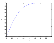
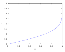
If a data distribution is approximately normal, then the proportion of data values within z standard deviations of the mean is defined by:

${\text{Proportion}}=\operatorname {erf} \left({\frac {z}{\sqrt {2}}}\right)$

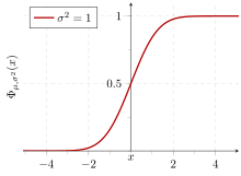
where $\textstyle \operatorname {erf}$ is the error function. The proportion that is less than or equal to a number, x, is given by the cumulative distribution function:^[16]

${\text{Proportion}}\leq x={\frac {1}{2}}\left[1+\operatorname {erf} \left({\frac {x-\mu }{\sigma {\sqrt {2}}}}\right)\right]={\frac {1}{2}}\left[1+\operatorname {erf} \left({\frac {z}{\sqrt {2}}}\right)\right].$

If a data distribution is approximately normal then about 68 percent of the data values are within one standard deviation of the mean (mathematically, μ ± σ, where μ is the arithmetic mean), about 95 percent are within two standard deviations (μ ± 2σ), and about 99.7 percent lie within three standard deviations (μ ± 3σ). This is known as the 68–95–99.7 rule, or the empirical rule.

For various values of z, the percentage of values expected to lie in and outside the symmetric interval, CI = (−zσ, zσ), are as follows:

Percentage within(z)

z(Percentage within)

Confidence interval	Proportion within	Proportion without
Percentage	Percentage	Fraction
0.318639σ	25%	75%	3 / 4
0.674490σ	50%	50%	1 / 2
0.977925σ	66.6667%	33.3333%	1 / 3
0.994458σ	68%	32%	1 / 3.125
1σ	68.2689492%	31.7310508%	1 / 3.1514872
1.281552σ	80%	20%	1 / 5
1.644854σ	90%	10%	1 / 10
1.959964σ	95%	5%	1 / 20
2σ	95.4499736%	4.5500264%	1 / 21.977895
2.575829σ	99%	1%	1 / 100
3σ	99.7300204%	0.2699796%	1 / 370.398
3.290527σ	99.9%	0.1%	1 / 1000
3.890592σ	99.99%	0.01%	1 / 10000
4σ	99.993666%	0.006334%	1 / 15787
4.417173σ	99.999%	0.001%	1 / 100000
4.5σ	99.9993204653751%	0.0006795346249%	1 / 147159.5358 6.8 / 1000000
4.891638σ	99.9999%	0.0001%	1 / 1000000
5σ	99.9999426697%	0.0000573303%	1 / 1744278
5.326724σ	99.99999%	0.00001%	1 / 10000000
5.730729σ	99.999999%	0.000001%	1 / 100000000
6σ	99.9999998027%	0.0000001973%	1 / 506797346
6.109410σ	99.9999999%	0.0000001%	1 / 1000000000
6.466951σ	99.99999999%	0.00000001%	1 / 10000000000
6.806502σ	99.999999999%	0.000000001%	1 / 100000000000
7σ	99.9999999997440%	0.000000000256%	1 / 390682215445

Relationship between standard deviation and mean[edit]

The mean and the standard deviation of a set of data are descriptive statistics usually reported together. In a certain sense, the standard deviation is a «natural» measure of statistical dispersion if the center of the data is measured about the mean. This is because the standard deviation from the mean is smaller than from any other point. The precise statement is the following: suppose x₁, …, x_n are real numbers and define the function:

$\sigma (r)={\sqrt {{\frac {1}{N-1}}\sum _{i=1}^{N}\left(x_{i}-r\right)^{2}}}.$

Using calculus or by completing the square, it is possible to show that σ(r) has a unique minimum at the mean:

$r={\bar {x}}.\,$

Variability can also be measured by the coefficient of variation, which is the ratio of the standard deviation to the mean. It is a dimensionless number.

Standard deviation of the mean[edit]

Often, we want some information about the precision of the mean we obtained. We can obtain this by determining the standard deviation of the sampled mean. Assuming statistical independence of the values in the sample, the standard deviation of the mean is related to the standard deviation of the distribution by:

$\sigma _{\text{mean}}={\frac {1}{\sqrt {N}}}\sigma$

where N is the number of observations in the sample used to estimate the mean. This can easily be proven with (see basic properties of the variance):

${\begin{aligned}\operatorname {var} (X)&\equiv \sigma _{X}^{2}\\\operatorname {var} (X_{1}+X_{2})&\equiv \operatorname {var} (X_{1})+\operatorname {var} (X_{2})\\\end{aligned}}$

(Statistical independence is assumed.)

$\operatorname {var} (cX_{1})\equiv c^{2}\,\operatorname {var} (X_{1})$

hence

${\begin{aligned}\operatorname {var} ({\text{mean}})&=\operatorname {var} \left({\frac {1}{N}}\sum _{i=1}^{N}X_{i}\right)={\frac {1}{N^{2}}}\operatorname {var} \left(\sum _{i=1}^{N}X_{i}\right)\\&={\frac {1}{N^{2}}}\sum _{i=1}^{N}\operatorname {var} (X_{i})={\frac {N}{N^{2}}}\operatorname {var} (X)={\frac {1}{N}}\operatorname {var} (X).\end{aligned}}$

Resulting in:

$\sigma _{\text{mean}}={\frac {\sigma }{\sqrt {N}}}.$

In order to estimate the standard deviation of the mean σ_mean it is necessary to know the standard deviation of the entire population σ beforehand. However, in most applications this parameter is unknown. For example, if a series of 10 measurements of a previously unknown quantity is performed in a laboratory, it is possible to calculate the resulting sample mean and sample standard deviation, but it is impossible to calculate the standard deviation of the mean. However, one can estimate the standard deviation of the entire population from the sample, and thus obtain an estimate for the standard error of the mean.

Rapid calculation methods[edit]

The following two formulas can represent a running (repeatedly updated) standard deviation. A set of two power sums s₁ and s₂ are computed over a set of N values of x, denoted as x₁, …, x_N:

$s_{j}=\sum _{k=1}^{N}{x_{k}^{j}}.$

Given the results of these running summations, the values N, s₁, s₂ can be used at any time to compute the current value of the running standard deviation:

$\sigma ={\frac {\sqrt {Ns_{2}-s_{1}^{2}}}{N}}$

Where N, as mentioned above, is the size of the set of values (or can also be regarded as s₀).

Similarly for sample standard deviation,

$s={\sqrt {\frac {Ns_{2}-s_{1}^{2}}{N(N-1)}}}.$

In a computer implementation, as the two s_j sums become large, we need to consider round-off error, arithmetic overflow, and arithmetic underflow. The method below calculates the running sums method with reduced rounding errors.^[17] This is a «one pass» algorithm for calculating variance of n samples without the need to store prior data during the calculation. Applying this method to a time series will result in successive values of standard deviation corresponding to n data points as n grows larger with each new sample, rather than a constant-width sliding window calculation.

For k = 1, …, n:

${\begin{aligned}A_{0}&=0\\A_{k}&=A_{k-1}+{\frac {x_{k}-A_{k-1}}{k}}\end{aligned}}$

where A is the mean value.

${\begin{aligned}Q_{0}&=0\\Q_{k}&=Q_{k-1}+{\frac {k-1}{k}}\left(x_{k}-A_{k-1}\right)^{2}=Q_{k-1}+\left(x_{k}-A_{k-1}\right)\left(x_{k}-A_{k}\right)\end{aligned}}$

Note: Q₁ = 0 since k − 1 = 0 or x₁ = A₁.

Sample variance:

$s_{n}^{2}={\frac {Q_{n}}{n-1}}$

Population variance:

$\sigma _{n}^{2}={\frac {Q_{n}}{n}}$

Weighted calculation[edit]

When the values x_i are weighted with unequal weights w_i, the power sums s₀, s₁, s₂ are each computed as:

$s_{j}=\sum _{k=1}^{N}w_{k}x_{k}^{j}.\,$

And the standard deviation equations remain unchanged. s₀ is now the sum of the weights and not the number of samples N.

The incremental method with reduced rounding errors can also be applied, with some additional complexity.

A running sum of weights must be computed for each k from 1 to n:

${\begin{aligned}W_{0}&=0\\W_{k}&=W_{k-1}+w_{k}\end{aligned}}$

and places where 1/σ is used above must be replaced by w_i/W_n:

${\begin{aligned}A_{0}&=0\\A_{k}&=A_{k-1}+{\frac {w_{k}}{W_{k}}}\left(x_{k}-A_{k-1}\right)\\Q_{0}&=0\\Q_{k}&=Q_{k-1}+{\frac {w_{k}W_{k-1}}{W_{k}}}\left(x_{k}-A_{k-1}\right)^{2}=Q_{k-1}+w_{k}\left(x_{k}-A_{k-1}\right)\left(x_{k}-A_{k}\right)\end{aligned}}$

In the final division,

$\sigma _{n}^{2}={\frac {Q_{n}}{W_{n}}}\,$

and

$s_{n}^{2}={\frac {Q_{n}}{W_{n}-1}},$

$s_{n}^{2}={\frac {n'}{n'-1}}\sigma _{n}^{2},$

where n is the total number of elements, and n′ is the number of elements with non-zero weights.

The above formulas become equal to the simpler formulas given above if weights are taken as equal to one.

History[edit]

The term standard deviation was first used in writing by Karl Pearson in 1894, following his use of it in lectures.^[18]^[19] This was as a replacement for earlier alternative names for the same idea: for example, Gauss used mean error.^[20]

Standard deviation index[edit]

The standard deviation index (SDI) is used in external quality assessments, particularly for medical laboratories. It is calculated as:^[21]

$SDI={\frac {Laboratory\ mean-Consensus\ group\ mean}{Consensus\ group\ standard\ deviation}}$

Higher dimensions[edit]

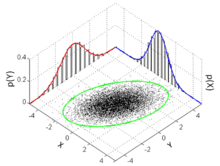
The standard deviation ellipse (green) of a two-dimensional normal distribution

In two dimensions, the standard deviation can be illustrated with the standard deviation ellipse (see Multivariate normal distribution § Geometric interpretation).

References[edit]

^ Bland, J.M.; Altman, D.G. (1996). «Statistics notes: measurement error». BMJ. 312 (7047): 1654. doi:10.1136/bmj.312.7047.1654. PMC 2351401. PMID 8664723.
^ Gauss, Carl Friedrich (1816). «Bestimmung der Genauigkeit der Beobachtungen». Zeitschrift für Astronomie und Verwandte Wissenschaften. 1: 187–197.
^ Walker, Helen (1931). Studies in the History of the Statistical Method. Baltimore, MD: Williams & Wilkins Co. pp. 24–25.
^ Weisstein, Eric W. «Bessel’s Correction». MathWorld.
^ «Standard Deviation Formulas». www.mathsisfun.com. Retrieved 21 August 2020.
^ Weisstein, Eric W. «Standard Deviation». mathworld.wolfram.com. Retrieved 21 August 2020.
^ «Consistent estimator». www.statlect.com. Retrieved 10 October 2022.
^ Gurland, John; Tripathi, Ram C. (1971), «A Simple Approximation for Unbiased Estimation of the Standard Deviation», The American Statistician, 25 (4): 30–32, doi:10.2307/2682923, JSTOR 2682923
^ «Standard Deviation Calculator». PureCalculators. 11 July 2021. Retrieved 14 September 2021.
^ Shiffler, Ronald E.; Harsha, Phillip D. (1980). «Upper and Lower Bounds for the Sample Standard Deviation». Teaching Statistics. 2 (3): 84–86. doi:10.1111/j.1467-9639.1980.tb00398.x.
^ Browne, Richard H. (2001). «Using the Sample Range as a Basis for Calculating Sample Size in Power Calculations». The American Statistician. 55 (4): 293–298. doi:10.1198/000313001753272420. JSTOR 2685690. S2CID 122328846.
^ «CERN experiments observe particle consistent with long-sought Higgs boson | CERN press office». Press.web.cern.ch. 4 July 2012. Archived from the original on 25 March 2016. Retrieved 30 May 2015.
^ LIGO Scientific Collaboration, Virgo Collaboration (2016), «Observation of Gravitational Waves from a Binary Black Hole Merger», Physical Review Letters, 116 (6): 061102, arXiv:1602.03837, Bibcode:2016PhRvL.116f1102A, doi:10.1103/PhysRevLett.116.061102, PMID 26918975, S2CID 124959784
^ «What is Standard Deviation». Pristine. Retrieved 29 October 2011.
^ Ghahramani, Saeed (2000). Fundamentals of Probability (2nd ed.). New Jersey: Prentice Hall. p. 438. ISBN 9780130113290.
^ Eric W. Weisstein. «Distribution Function». MathWorld. Wolfram. Retrieved 30 September 2014.
^ Welford, B. P. (August 1962). «Note on a Method for Calculating Corrected Sums of Squares and Products». Technometrics. 4 (3): 419–420. CiteSeerX 10.1.1.302.7503. doi:10.1080/00401706.1962.10490022.
^ Dodge, Yadolah (2003). The Oxford Dictionary of Statistical Terms. Oxford University Press. ISBN 978-0-19-920613-1.
^ Pearson, Karl (1894). «On the dissection of asymmetrical frequency curves». Philosophical Transactions of the Royal Society A. 185: 71–110. Bibcode:1894RSPTA.185…71P. doi:10.1098/rsta.1894.0003.
^ Miller, Jeff. «Earliest Known Uses of Some of the Words of Mathematics».
^ Harr, Robert R. (2012). Medical laboratory science review. Philadelphia: F. A. Davis Co. p. 236. ISBN 978-0-8036-3796-2. OCLC 818846942.

External links[edit]

«Quadratic deviation», Encyclopedia of Mathematics, EMS Press, 2001 [1994]
«Standard Deviation Calculator»

Источник

Я читаю курс статистического мышления магистрам, и одна тема вызывает у них явные затруднения – чем стандартное отклонение отличается от стандартной ошибки, и в каких случаях, применять ту или иную статистику. А недавно в книге Искусство статистики Дэвида Шпигельхалтера я узнал про бутстрэппинг, и понял, как объяснить различия стандартного отклонения и стандартной ошибки.

Для начала зададим 100 значений стандартной нормально распределенной случайной величины. В этом контексте стандартная означает, что ее матожидание μ = 0, а среднеквадратичное отклонение σ = 1. Поскольку значения в Excel получены с помощью волатильной функции СЛМАССИВ(), после любого действия они пересчитываются. Поэтому диаграммы в заметке и в файле будут отличаться.

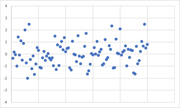
Рис. 1. Нормально распределенная случайная величина

Скачать заметку в формате Word или pdf, примеры в формате Excel

Стандартное отклонение

… является наиболее распространенным показателем рассеивания значений случайной величины относительно её среднего арифметического.

Стандартное отклонение вычисляют по формуле:

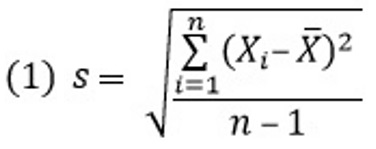
где X̅ – среднее арифметическое значений случайной величины (далее я буду называть его просто средним), Х_i – отдельные значения случайной величины, n – число значений случайной величины.

Вообще термины разными авторами используются немного по-разному. Мне нравится следующий подход. Генеральную совокупность описывают параметрами, обозначаемыми греческими буквами: математическое ожидание μ и среднеквадратичное отклонение σ. Выборки описывают статистиками, обозначаемыми латинскими буквами: среднее арифметическое X̅ и стандартное отклонение s. Стандартное отклонение иначе называют оценкой среднеквадратичного отклонения. Как правило, есть генеральная совокупность с неизвестным нам среднеквадратичным отклонением σ. Извлекая выборку, и вычисляя стандартное отклонение s, мы кое-что узнаем о среднеквадратичном отклонении генеральной совокупности σ. Поэтому и говорят, что s является оценкой сигмы.

На самом деле за термином стандартное отклонение стоят две немного отличающиеся статистики. Но эта заметка о другом)) Подробнее см. СТАНДОТКЛОН.В и СТАНДОТКЛОН.Г: в чем различие?

Нанесем на диаграмму линию среднего и границы, отстоящие от среднего на расстоянии ±2s.

Рис. 2. Линия среднего и границы ±2s

Для стандартного нормального распределения за границы ±2s попадают 4,6% значений.

=(1-НОРМ.СТ.РАСП(2;ИСТИНА))*2 = 4,6%

И действительно 5 точек на рис. 2 лежат вне границ. Совпадение не обязано быть таким точным. Если вы откроете файл Excel на листе «Рис. 2» и понажимаете F9, принудительно изменяя случайные значения, то увидите, что вне границ может лежать от 2 до 8 точек. А если нажимать F9 достаточно долго, то вы получите более экстремальные числа точек вне границ. Для стандартного нормального распределения в пределах ±2s лежат приблизительно 95% значений. Поскольку s – оценка среднеквадратичного отклонения σ, которое в свою очередь равно 1, то 95% всех значений попадают в диапазон ≈ ±2.

Чем меньше s, тем кучнее значения случайной величины располагаются вокруг среднего. Итак

стандартное отклонение – мера разброса случайной величины

Среднее арифметическое выборки

Напомню, что мы задаем наши 100 значений с помощью генератора случайных чисел формулой в Excel

=НОРМ.СТ.ОБР(СЛМАССИВ(100;;0;1;ЛОЖЬ))

Хотя мы установили для генератора случайных чисел μ = 0 и σ = 1, значения X̅ и s будут немного отличаться для каждой выборки.

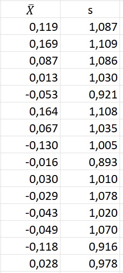
Рис. 3. Среднее и стандартное отклонение для 15 выборок размером n = 100

Теперь мы хотим узнать, что можно сказать о неизвестном математическом ожидании генеральной совокупности μ, подсчитав среднее арифметическое конкретной выборки, например, первой X̅ = 0,119?

Бутстрэп

Как пишет Евгения Поникарова, переводчик книги Дэвида Шпигельхалтера «Искусство статистики», слово bootstraps означает ремешки в виде ушка, которые прикрепляются к верхней части обуви, чтобы ее было проще натягивать. В английском языке есть выражение To pull oneself over a fence by one’s bootstraps (буквально — перетащить себя через ограду за ушки своей обуви), которое означает «выпутаться из своих проблем самому». Еще можно вспомнить барона Мюнхгаузена, который вытащил себя за волосы из болота.

Бутстрэп – компьютерный метод исследования распределения статистик, основанный на многократной генерации выборок методом Монте-Карло на базе имеющейся одной выборки. Термин ввел в 1977 году Брэдли Эфрон.

Итак, возьмем одну выборку из 100 случайных чисел и зафиксируем значения. Это наша исходная выборка (столбец А на рис. 4). Её среднее X̅(100) = 0,121, а стандартное отклонение s(100) = 0,995. 95% значений попадают в диапазон ≈ 0,121 ± 1,990.

С помощью генератора случайных чисел будем формировать из исходной выборки бутстрэп-выборки разного размера. Хитрость заключается в том, что выбирать значения мы будем с возвращением. Т.е., все значения любой бутстрэп-выборки взяты из исходной, а вот уникальность значений будет потеряна. Например, выборка в столбце С содержит два значения 0,7394. Я подсветил их с помощью условного форматирования. Опять же, если вы откроете Excel-файл, то дублей может не быть, так как бутстрэп-выборка сформирована волатильной функцией СЛМАССИВ().

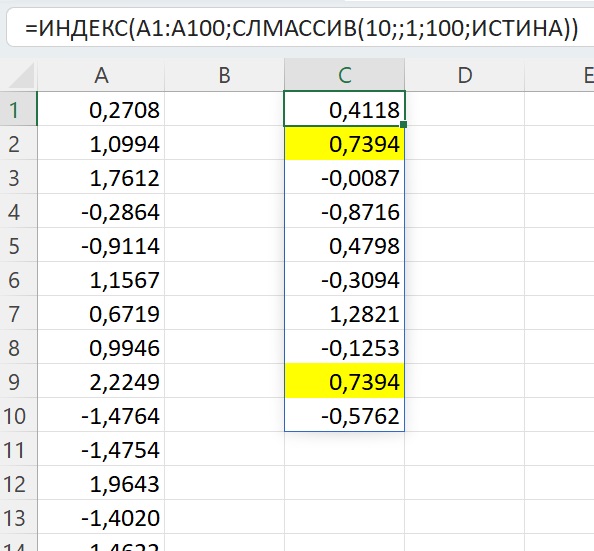
Рис. 4. Бутстрэп-выборка может содержать повторения

Для удобства последующей обработки расположим значения бутстрэп-выборки по горизонтали. Начнем со значения n = 3. Извлечем 1000 бутстрэп-выборок (рис. 5). В столбце А исходная выборка, n = 100. Столбец С содержит номер бутстрэп-выборки. В столбцах D, E и F извлеченные значения, в G – средние значения по выборкам. В ячейке G1 среднее D1:F1, в ячейке G2 – среднее D2:F2 и т.д. На диаграмме показано распределение средних значений бутстрэп-выборок для n = 3.

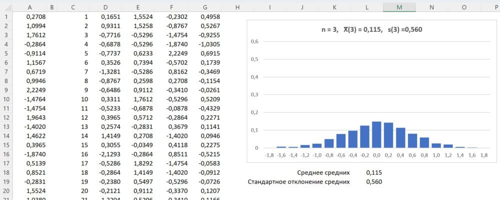
Рис. 5. Распределений средних значений 1000 бутстрэп-выборок, n = 3

Среднее средних 1000 бутстрэп-выборок = 0,115, стандартное отклонение средних значений 1000 бутстрэп-выборок = 0,560. Напоминаю, что 95% исходных значений выборки попадают в диапазон 0,12 ± 1,99. Для бутстрэп-выборок n = 3 мы только что нашли, что 95% средних попадают в диапазон 0,115 ± 1,120 (0,560*2 = 1,120). Кажется естественным, что разброс средних меньше, чем разброс отдельных значений.

Повторим моделирование для n = 5, 20, 50.

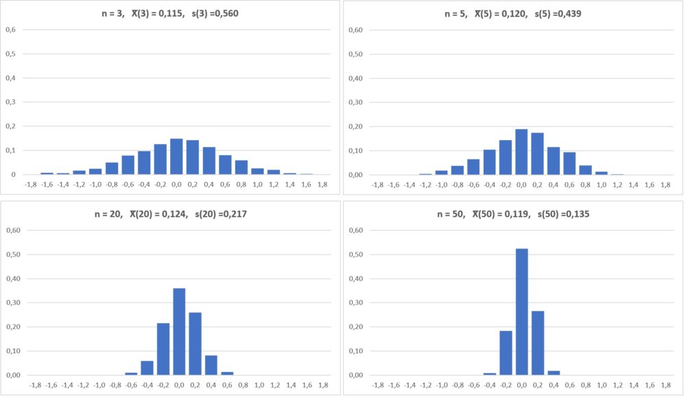
Рис. 6. С увеличением n стандартное отклонение средних значений бутстрэп-выборок уменьшается

Осмыслим, что мы получили. На рис. 6 представлены распределения средних значений бутстрэп-выборок разного размера из исходной выборки 100 случайных нормально распределенных чисел. Среднее каждого распределения близко к нулю (в нашей конкретной выборке из 100 чисел это среднее равно 0,121). А вот стандартное отклонение s(n) уменьшается по мере роста размера бутстрэп-выборок: s(3) = 0,560, s(5) = 0,439, s(20) = 0,217, s(50) = 0,135.

Стандартна ошибка

…или стандартная ошибка среднего – статистика, характеризующая стандартное отклонение выборочного среднего, рассчитанное по выборке размера n из генеральной совокупности.

Ничего не напоминает!? А что за статистику s(n) мы рассчитали выше в бутстрэп-анализе!? Да, это было стандартное отклонение выборочного среднего X̅(n).

Величина стандартной ошибки зависит от дисперсии генеральной совокупности σ² и объёма выборки n. Стандартная ошибка среднего вычисляется по формуле

где σ – величина среднеквадратического отклонения генеральной совокупности, и n – объём выборки. Поскольку дисперсия генеральной совокупности, как правило, неизвестна, то оценка стандартной ошибки вычисляется по формуле:

где s — стандартное отклонение случайной величины.

Сведем в одной таблице рассмотренные статистики:

Рис. 7. Рассмотренные статистики

Здесь в столбцах J:L приведены статистики для одной выборки размера n, а в столбце M – статистики для бутстрэп-выборок соответствующего размера с рис. 6. Если в Excel-файле на листе «Рис. 7» понажимать F9, вы увидите, что не всегда совпадение между столбцами L и M будет таким хорошим, но тенденция будет прослеживаться.

Выше я писал, что мы исследуем неизвестное математическое ожидание генеральной совокупности μ на основе среднего арифметического выборки X̅(100) = 0,119.

Мы можем использовать статистику, именуемую стандартной ошибкой. Для нас она черный ящик – формула, выведенная на основе теории вероятностей. С другой стороны мы можем построить множество бутстрэп-выборок размера n = 100, и подсчитать стандартное отклонение средних этих бутстрэп-выборок. И мы показали, что стандартная ошибка для одной выборки и стандартное отклонение средних бутстрэп-выборок, это одно и то же! В нашем примере, получив X̅(100) = 0,119, мы можем сказать, что с вероятностью 95% математическое ожидание генеральной совокупности μ лежит в диапазоне 0,119 ± 0,212 (0,106*2=0,212). Итак

стандартная ошибка – мера оценки математического ожидания генеральной совокупности μ на основании статистик выборки

Например, 95%-ный доверительный интервал для μ

Понятно, что с увеличением размера выборки n доверительный интервал будет сужаться. В пределе при n → ∞, X̅ → μ и SE → 0.

Источник

Стандартное отклонение и стандартная ошибка: в чем разница?

17 авг. 2022 г.
читать 2 мин

В статистике студенты часто путают два термина: стандартное отклонение и стандартная ошибка .

Стандартное отклонение измеряет, насколько разбросаны значения в наборе данных.

Стандартная ошибка — это стандартное отклонение среднего значения в повторных выборках из совокупности.

Давайте рассмотрим пример, чтобы ясно проиллюстрировать эту идею.

Пример: стандартное отклонение против стандартной ошибки

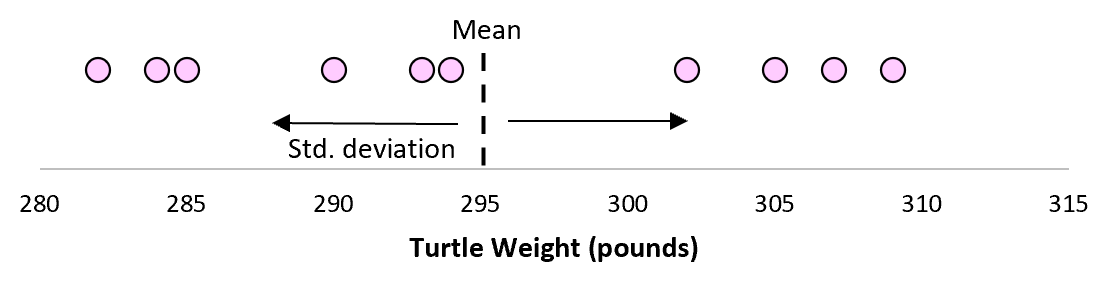
Предположим, мы измеряем вес 10 разных черепах.

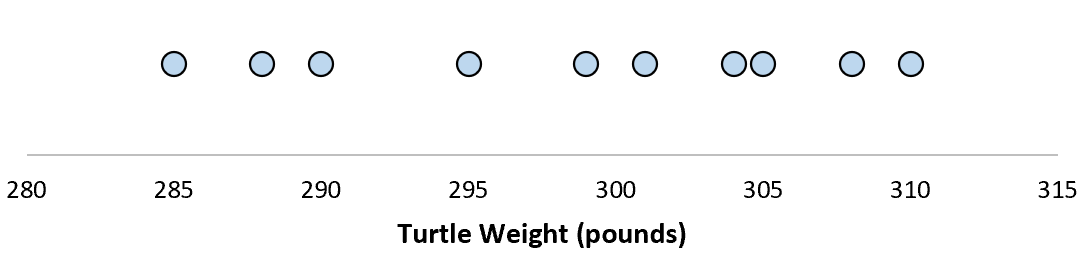
Для этой выборки из 10 черепах мы можем вычислить среднее значение выборки и стандартное отклонение выборки:

Предположим, что стандартное отклонение оказалось равным 8,68. Это дает нам представление о том, насколько распределен вес этих черепах.

Но предположим, что мы собираем еще одну простую случайную выборку из 10 черепах и также проводим их измерения. Более чем вероятно, что эта выборка из 10 черепах будет иметь немного другое среднее значение и стандартное отклонение, даже если они взяты из одной и той же популяции:

Теперь, если мы представим, что мы берем повторные выборки из одной и той же совокупности и записываем выборочное среднее и выборочное стандартное отклонение для каждой выборки:

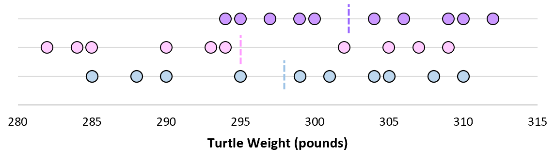
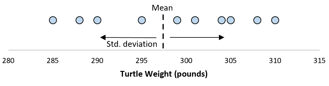
Теперь представьте, что мы наносим каждое среднее значение выборки на одну и ту же строку:

Стандартное отклонение этих средних значений известно как стандартная ошибка.

Формула для фактического расчета стандартной ошибки:

Стандартная ошибка = s/ √n

куда:

s: стандартное отклонение выборки
n: размер выборки

Какой смысл использовать стандартную ошибку?

Когда мы вычисляем среднее значение данной выборки, нас на самом деле интересует не среднее значение этой конкретной выборки, а скорее среднее значение большей совокупности, из которой взята выборка.

Однако мы используем выборки, потому что для них гораздо проще собирать данные, чем для всего населения. И, конечно же, среднее значение выборки будет варьироваться от выборки к выборке, поэтому мы используем стандартную ошибку среднего значения как способ измерить, насколько точна наша оценка среднего значения.

Вы заметите из формулы для расчета стандартной ошибки, что по мере увеличения размера выборки (n) стандартная ошибка уменьшается:

Стандартная ошибка = s/ √n

Это должно иметь смысл, поскольку большие размеры выборки уменьшают изменчивость и увеличивают вероятность того, что среднее значение нашей выборки ближе к фактическому среднему значению генеральной совокупности.

Когда использовать стандартное отклонение против стандартной ошибки

Если мы просто заинтересованы в измерении того, насколько разбросаны значения в наборе данных, мы можем использовать стандартное отклонение .

Однако, если мы заинтересованы в количественной оценке неопределенности оценки среднего значения, мы можем использовать стандартную ошибку среднего значения .

В зависимости от вашего конкретного сценария и того, чего вы пытаетесь достичь, вы можете использовать либо стандартное отклонение, либо стандартную ошибку.

Источник

Основы теории контроля качества.

Основные статистические понятия, используемые в контроле качества.

Использование и интерпретация величины среднеквадратического отклонения

Расчет среднеквадратичного (стандартного) отклонения

Формулы вычисления стандартного отклонения

Разница между формулами S и σ («n» и «n–1»)

Как рассчитать стандартное отклонение?

Пример 1 (с σ)

Пример 2 (с S)

Дисперсия и стандартное отклонение

Правило трёх сигм

Стандартное отклонение в excel

Коэффициент вариации

Basic examples[edit]

Population standard deviation of grades of eight students[edit]

Standard deviation of average height for adult men[edit]

Definition of population values[edit]

Discrete random variable[edit]

Continuous random variable[edit]

Estimation[edit]

Uncorrected sample standard deviation[edit]

Corrected sample standard deviation[edit]

Unbiased sample standard deviation[edit]

Confidence interval of a sampled standard deviation[edit]

Bounds on standard deviation[edit]

Identities and mathematical properties[edit]

Interpretation and application[edit]

Application examples[edit]

Experiment, industrial and hypothesis testing[edit]

Weather[edit]

Finance[edit]

Geometric interpretation[edit]

Chebyshev’s inequality[edit]

Rules for normally distributed data[edit]

Relationship between standard deviation and mean[edit]

Standard deviation of the mean[edit]

Rapid calculation methods[edit]

Weighted calculation[edit]

History[edit]

Standard deviation index[edit]

Higher dimensions[edit]

See also[edit]

References[edit]

External links[edit]

Стандартное отклонение

Среднее арифметическое выборки

Бутстрэп

Стандартна ошибка

Стандартное отклонение и стандартная ошибка: в чем разница?

Пример: стандартное отклонение против стандартной ошибки

Какой смысл использовать стандартную ошибку?

Когда использовать стандартное отклонение против стандартной ошибки