- numpy.std(a, axis=None, dtype=None, out=None, ddof=0, keepdims=<no value>, *, where=<no value>)[source]#
-
Compute the standard deviation along the specified axis.
Returns the standard deviation, a measure of the spread of a distribution,
of the array elements. The standard deviation is computed for the
flattened array by default, otherwise over the specified axis.- Parameters:
-
- aarray_like
-
Calculate the standard deviation of these values.
- axisNone or int or tuple of ints, optional
-
Axis or axes along which the standard deviation is computed. The
default is to compute the standard deviation of the flattened array.New in version 1.7.0.
If this is a tuple of ints, a standard deviation is performed over
multiple axes, instead of a single axis or all the axes as before. - dtypedtype, optional
-
Type to use in computing the standard deviation. For arrays of
integer type the default is float64, for arrays of float types it is
the same as the array type. - outndarray, optional
-
Alternative output array in which to place the result. It must have
the same shape as the expected output but the type (of the calculated
values) will be cast if necessary. - ddofint, optional
-
Means Delta Degrees of Freedom. The divisor used in calculations
isN - ddof, whereNrepresents the number of elements.
By default ddof is zero. - keepdimsbool, optional
-
If this is set to True, the axes which are reduced are left
in the result as dimensions with size one. With this option,
the result will broadcast correctly against the input array.If the default value is passed, then keepdims will not be
passed through to thestdmethod of sub-classes of
ndarray, however any non-default value will be. If the
sub-class’ method does not implement keepdims any
exceptions will be raised. - wherearray_like of bool, optional
-
Elements to include in the standard deviation.
Seereducefor details.New in version 1.20.0.
- Returns:
-
- standard_deviationndarray, see dtype parameter above.
-
If out is None, return a new array containing the standard deviation,
otherwise return a reference to the output array.
Notes
The standard deviation is the square root of the average of the squared
deviations from the mean, i.e.,std = sqrt(mean(x)), where
x = abs(a - a.mean())**2.The average squared deviation is typically calculated as
x.sum() / N,
whereN = len(x). If, however, ddof is specified, the divisor
N - ddofis used instead. In standard statistical practice,ddof=1
provides an unbiased estimator of the variance of the infinite population.
ddof=0provides a maximum likelihood estimate of the variance for
normally distributed variables. The standard deviation computed in this
function is the square root of the estimated variance, so even with
ddof=1, it will not be an unbiased estimate of the standard deviation
per se.Note that, for complex numbers,
stdtakes the absolute
value before squaring, so that the result is always real and nonnegative.For floating-point input, the std is computed using the same
precision the input has. Depending on the input data, this can cause
the results to be inaccurate, especially for float32 (see example below).
Specifying a higher-accuracy accumulator using thedtypekeyword can
alleviate this issue.Examples
>>> a = np.array([[1, 2], [3, 4]])
>>> np.std(a)
1.1180339887498949 # may vary
>>> np.std(a, axis=0)
array([1.,  1.])
>>> np.std(a, axis=1)
array([0.5,  0.5])
In single precision, std() can be inaccurate:
>>> a = np.zeros((2, 512*512), dtype=np.float32)
>>> a[0, :] = 1.0
>>> a[1, :] = 0.1
>>> np.std(a)
0.45000005
Computing the standard deviation in float64 is more accurate:
>>> np.std(a, dtype=np.float64)
0.44999999925494177 # may vary
Specifying a where argument:
>>> a = np.array([[14, 8, 11, 10], [7, 9, 10, 11], [10, 15, 5, 10]])
>>> np.std(a)
2.614064523559687 # may vary
>>> np.std(a, where=[[True], [True], [False]])
2.0
The standard error of the mean is a way to measure how spread out values are in a dataset. It is calculated as:
Standard error of the mean = s / √n
where:
- s: sample standard deviation
- n: sample size
This tutorial explains two methods you can use to calculate the standard error of the mean for a dataset in Python. Note that both methods produce the exact same results.
Method 1: Use SciPy
The first way to calculate the standard error of the mean is to use the sem() function from the SciPy Stats library.
The following code shows how to use this function:
from scipy.stats import sem

#define dataset
data = [3, 4, 4, 5, 7, 8, 12, 14, 14, 15, 17, 19, 22, 24, 24, 24, 25, 28, 28, 29]

#calculate standard error of the mean
sem(data)

2.001447
The standard error of the mean turns out to be 2.001447.
Method 2: Use NumPy
Another way to calculate the standard error of the mean for a dataset is to use the std() function from NumPy.
Note that we must specify ddof=1 in the argument for this function to calculate the sample standard deviation as opposed to the population standard deviation.
The following code shows how to do so:
import numpy as np

#define dataset
data = np.array([3, 4, 4, 5, 7, 8, 12, 14, 14, 15, 17, 19, 22, 24, 24, 24, 25, 28, 28, 29])

#calculate standard error of the mean
np.std(data, ddof=1) / np.sqrt(np.size(data))

2.001447
Once again, the standard error of the mean turns out to be 2.001447.
How to Interpret the Standard Error of the Mean
The standard error of the mean is simply a measure of how spread out values are around the mean. There are two things to keep in mind when interpreting the standard error of the mean:
1. The larger the standard error of the mean, the more spread out values are around the mean in a dataset.
To illustrate this, consider if we change the last value in the previous dataset to a much larger number:
from scipy.stats import sem

#define dataset
data = [3, 4, 4, 5, 7, 8, 12, 14, 14, 15, 17, 19, 22, 24, 24, 24, 25, 28, 28, 150]

#calculate standard error of the mean
sem(data)

6.978265
Notice how the standard error jumps from 2.001447 to 6.978265. This is an indication that the values in this dataset are more spread out around the mean compared to the previous dataset.
2. As the sample size increases, the standard error of the mean tends to decrease.
To illustrate this, consider the standard error of the mean for the following two datasets:
from scipy.stats import sem

#define first dataset and find SEM
data1 = [1, 2, 3, 4, 5]
sem(data1)

0.7071068

#define second dataset and find SEM
data2 = [1, 2, 3, 4, 5, 1, 2, 3, 4, 5]
sem(data2)

0.4714045
The second dataset is simply the first dataset repeated twice. Thus, the two datasets have the same mean but the second dataset has a larger sample size so it has a smaller standard error.
Additional Resources
How to Calculate the Standard Error of the Mean in R
How to Calculate the Standard Error of the Mean in Excel
How to Calculate Standard Error of the Mean in Google Sheets
numpy.std(arr, axis = None) : Compute the standard deviation of the given data (array elements) along the specified axis(if any)..
Standard Deviation (SD) is measured as the spread of data distribution in the given data set.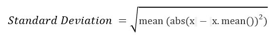
For example :
x = 1 1 1 1 1
Standard Deviation = 0 .

y = 9, 2, 5, 4, 12, 7, 8, 11, 9, 3, 7, 4, 12, 5, 4, 10, 9, 6, 9, 4
Step 1 : Mean of distribution 4 = 7
Step 2 : Summation of (x - x.mean())**2 = 178
Step 3 : Finding Mean = 178 /20 = 8.9
This Result is Variance.
Step 4 : Standard Deviation = sqrt(Variance) = sqrt(8.9) = 2.983..
Parameters :
arr : [array_like]input array.
axis : [int or tuples of int]axis along which we want to calculate the standard deviation. Otherwise, it will consider arr to be flattened (works on all the axis). axis = 0 means SD along the column and axis = 1 means SD along the row.
out : [ndarray, optional]Different array in which we want to place the result. The array must have the same dimensions as expected output.
dtype : [data-type, optional]Type we desire while computing SD.Results : Standard Deviation of the array (a scalar value if axis is none) or array with standard deviation values along specified axis.
Code #1:
import numpy as np
arr = [20, 2, 7, 1, 34]
print("arr : ", arr)
print("std of arr : ", np.std(arr))
print ("\nMore precision with float32")
print("std of arr : ", np.std(arr, dtype = np.float32))
print ("\nMore accuracy with float64")
print("std of arr : ", np.std(arr, dtype = np.float64))
Output :
arr :  [20, 2, 7, 1, 34]
std of arr :  12.576167937809991

More precision with float32
std of arr :  12.576168

More accuracy with float64
std of arr :  12.576167937809991
Code #2:
import numpy as np
arr = [[2, 2, 2, 2, 2],
[15, 6, 27, 8, 2],
[23, 2, 54, 1, 2, ],
[11, 44, 34, 7, 2]]
print("\nstd of arr, axis = None : ", np.std(arr))
print("\nstd of arr, axis = 0 : ", np.std(arr, axis = 0))
print("\nstd of arr, axis = 1 : ", np.std(arr, axis = 1))
Output :
std of arr, axis = None :  15.3668474320532

std of arr, axis = 0 :  [ 7.56224173 17.68473918 18.59267329  3.04138127  0.        ]

std of arr, axis = 1 :  [ 0.          8.7772433  20.53874388 16.40243884]
Last Updated :
28 Nov, 2018
Like Article
Save Article
Стандартная ошибка среднего — это способ измерить, насколько разбросаны значения в наборе данных. Он рассчитывается как:
Стандартная ошибка среднего = s / √n
куда:
- s : стандартное отклонение выборки
- n : размер выборки
В этом руководстве объясняются два метода, которые вы можете использовать для вычисления стандартной ошибки среднего значения для набора данных в Python. Обратите внимание, что оба метода дают одинаковые результаты.
Способ 1: используйте SciPy
Первый способ вычислить стандартную ошибку среднего — использовать функцию sem() из библиотеки SciPy Stats.
Следующий код показывает, как использовать эту функцию:
from scipy. stats import sem

#define dataset
data = [3, 4, 4, 5, 7, 8, 12, 14, 14, 15, 17, 19, 22, 24, 24, 24, 25, 28, 28, 29]

#calculate standard error of the mean
sem(data)

2.001447
Стандартная ошибка среднего оказывается равной 2,001447 .
Способ 2: использовать NumPy
Другой способ вычислить стандартную ошибку среднего для набора данных — использовать функцию std() из NumPy.
Обратите внимание, что мы должны указать ddof=1 в аргументе этой функции, чтобы вычислить стандартное отклонение выборки, а не стандартное отклонение генеральной совокупности.
Следующий код показывает, как это сделать:
import numpy as np

#define dataset
data = np.array([3, 4, 4, 5, 7, 8, 12, 14, 14, 15, 17, 19, 22, 24, 24, 24, 25, 28, 28, 29])

#calculate standard error of the mean
np.std(data, ddof= 1 ) / np.sqrt (np.size (data))

2.001447
И снова стандартная ошибка среднего оказывается равной 2,001447 .
Как интерпретировать стандартную ошибку среднего
Стандартная ошибка среднего — это просто мера того, насколько разбросаны значения вокруг среднего. При интерпретации стандартной ошибки среднего следует помнить о двух вещах:
1. Чем больше стандартная ошибка среднего, тем более разбросаны значения вокруг среднего в наборе данных.
Чтобы проиллюстрировать это, рассмотрим, изменим ли мы последнее значение в предыдущем наборе данных на гораздо большее число:
from scipy. stats import sem

#define dataset
data = [3, 4, 4, 5, 7, 8, 12, 14, 14, 15, 17, 19, 22, 24, 24, 24, 25, 28, 28, 150 ]

#calculate standard error of the mean
sem(data)

6.978265
Обратите внимание на скачок стандартной ошибки с 2,001447 до 6,978265.Это указывает на то, что значения в этом наборе данных более разбросаны вокруг среднего значения по сравнению с предыдущим набором данных.
2. По мере увеличения размера выборки стандартная ошибка среднего имеет тенденцию к уменьшению.
Чтобы проиллюстрировать это, рассмотрим стандартную ошибку среднего для следующих двух наборов данных:
from scipy.stats import sem

#define first dataset and find SEM
data1 = [1, 2, 3, 4, 5]
sem(data1)

0.7071068

#define second dataset and find SEM
data2 = [1, 2, 3, 4, 5, 1, 2, 3, 4, 5]
sem(data2)

0.4714045
Второй набор данных — это просто первый набор данных, повторенный дважды. Таким образом, два набора данных имеют одинаковое среднее значение, но второй набор данных имеет больший размер выборки, поэтому стандартная ошибка меньше.
Дополнительные ресурсы
Как рассчитать стандартную ошибку среднего в R
Как рассчитать стандартную ошибку среднего в Excel
Как рассчитать стандартную ошибку среднего в Google Sheets
The Standard Error of the Mean (SEM) describes how far a sample mean varies from the actual population mean.
It is used to estimate the approximate confidence intervals for the mean.
In this tutorial, we will discuss two methods you can use to calculate the Standard Error of the Mean in python with step-by-step examples.
The Standard error of the mean for a sample is calculated using below formula:
Standard error of the mean (SEM) = s / √n
where:
s : sample standard deviation
n : sample size
Method 1: Use Numpy
We will be using the numpy available in python, it provides std() function to calculate the standard error of the mean.
If you don’t have numpy package installed, use the below command on windows command prompt for numpy library installation.
pip install numpy
Example 1: How to calculate SEM in Python
Let’s understand, how to calculate the standard error of mean (SEM) with the given below python code.
#import modules
import numpy as np

#define dataset
data = np.array([4,7,3,9,12,8,14,10,12,12])

#calculate standard error of the mean
result = np.std(data, ddof=1) / np.sqrt(np.size(data))

#Print the result
print("The Standard error of the mean : %.3f"%result)
In the above code, we import numpy library to define the dataset.
Using std() function we calculated the standard error of the mean.
Note that we must specify ddof=1 in the argument for std() function to calculate the sample standard deviation instead of population standard deviation.
The Output of the above code is shown below.
#Output
The Standard error of the mean : 1.149
The Standard error of the mean is 1.149.
Method 2: Use Scipy
We will be using Scipy library available in python, it provides sem() function to calculate the standard error of the mean.
If you don’t have the scipy library installed then use the below command on windows command prompt for scipy library installation.
pip install scipy
Example 2: How to calculate SEM in Python
Lets assume we have dataset as below
data = [4,7,3,9,12,8,14,10,12,12]
Lets calculate the standard error of mean by using below python code.
#import modules
import scipy.stats as stat

#define dataset
data = [4,7,3,9,12,8,14,10,12,12]

#calculate standard error of the mean
result = stat.sem(data)

#Print the result
print("The Standard error of the mean : %.3f"%result)
In the above code, we import numpy library to define the dataset.
Using sem() function we calculated the standard error of the mean.
The Output of the above code is shown below.
#Output
The Standard error of the mean : 1.149
How to Interpret the Standard Error of the Mean
The two important factors to keep in mind while interpreting the SEM are as follows:-
1 Sample Size:- With the increase in sample size, the standard error of mean tends to decrease.
Let’s see this with below example:-
#import modules
import scipy.stats as stat

#define dataset 1
data1 = [4,7,3,9,12,8,14,10,12,12]

#define dataset 2 by repeated the first dataset twice
data2 = [4,7,3,9,12,8,14,10,12,12,4,7,3,9,12,8,14,10,12,12]

#calculate standard error of the mean
result1 = stat.sem(data1)
result2 = stat.sem(data2)

#Print the result
print("The Standard error of the mean for the original dataset: %.3f"%result1)
print("The Standard error of the mean for the repeated dataset : %.3f"%result2)
In the above example, we created the two datasets i.e. data1 & data2 where data2 is just the twice of data1.
The Output of the above code is shown below:-
# Output
The Standard error of the mean for the original dataset: 1.149
The Standard error of the mean for the repeated dataset : 0.791
We seen that for data1 the SEM is 1.149 and for data2 SEM is 0.791.
It clearly shows that with an increase in size the SEM decreases.
Values of data2 are less spread out around the mean as compared to data1, although both have the same mean value.
2 The Value of SEM : The larger value of the SEM indicates that the values are more spread around the mean .
Let’s discuss this with below example:-
#import modules
import scipy.stats as stat

#define dataset 1
data1 = [4,7,3,9,12,8,14,10,12,12]

#define dataset 2 by replace last value with 120
data2 = [4,7,3,9,12,8,14,10,12,120]

#calculate standard error of the mean
result1 = stat.sem(data1)
result2 = stat.sem(data2)

#Print the result
print("The Standard error of the mean for the original dataset: %.3f"%result1)
print("The Standard error of the mean for the repeated dataset : %.3f"%result2)
In the above example, we created the two datasets i.e. data1 & data2 where data2 is created by replacing the last value with 120.
The Output of the above code is shown below:-
#Output
The Standard error of the mean for the original dataset: 1.149
The Standard error of the mean for the repeated dataset : 11.177
We seen that for data1 the SEM is 1.149 and for data2 SEM is 11.177.
It clearly shows that SEM for data2 is larger as compared to data1.
It means the values of data2 are more spread out around the mean as compared to data1.
Conclusion
I hope, you may find how to calculate the Standard Error of the Mean in the python tutorial with a step-by-step illustration of examples educational and helpful.

Is it gonna rain today? Should I take my umbrella to the office or not? To know the answer to such questions we will just take out our phone and check the weather forecast. How is this done? There are computer models which use statistics to compare weather conditions from the past with the current conditions to predict future weather conditions. From studying the amount of fluoride that is safe in our toothpaste to predicting the future stock rates, everything requires statistics. Data is everything in statistics. Calculating the range, median, and mode of the data set is all a part of descriptive statistics.
Data representation, manipulation, and visualization are key components in statistics. You can read about it here.
The next important step is analyzing the data, which can be done using both descriptive and inferential statistics. Both descriptive and inferential statistics are used to analyze results and draw conclusions in most of the research studies conducted on groups of people.
Through this article, we will learn descriptive statistics using python.

Introduction
Descriptive statistics describe the basic and important features of data. Descriptive statistics help simplify and summarize large amounts of data in a sensible manner. For instance, consider the Cumulative Grade Point Index (CGPI), which is used to describe the general performance of a student across a wide range of course experiences.
Descriptive statistics involve evaluating measures of center(centrality measures) and measures of dispersion(spread).

Centrality measures
Centrality measures give us an estimate of the center of a distribution. It gives us a sense of a typical value we would expect to see. The three major measures of center include the mean, median, and mode.
- Mean means…
…the average of the given values. To compute mean, sum all the values and divide the sum by the number of values.
(displaystyleoverline{x}=frac{1}{n}sum_{i=1}^n x_i)
Consider a class of 7 students. Suppose they appear for midterm exams and score the following marks out of 20:
Name Subject 1 Subject 2 Subject 3 Subject 4 Total Marks Student 1 10 8 15 11.5 44.5 Student 2 14 9 7.5 11 41.5 Student 3 11 17 11.5 9 48.5 Student 4 7 14.5 10 12 43.5 Student 5 9.5 12 10.5 14 46 Student 6 15 18 7 12 52 Student 7 19 15.5 11 7.5 53 
Mean for Subject 1 Mean with python
There are various libraries in python such as pandas, numpy, statistics (Python version 3.4) that support mean calculation.
numpy.mean(a, axis=None, dtype=None)
a: array containing numbers whose mean is required
axis: axis or axes along which the means are computed, default is to compute the mean of the flattened array
dtype: type of data to be used in calculations>>> import numpy as np >>> A = np.array([[10,14,11,7,9.5,15,19],[8,9,17,14.5,12,18,15.5], [15,7.5,11.5,10,10.5,7,11],[11.5,11,9,12,14,12,7.5]]) >>> B = A.T >>> print B [[ 10. 8. 15. 11.5] [ 14. 9. 7.5 11. ] [ 11. 17. 11.5 9. ] [ 7. 14.5 10. 12. ] [ 9.5 12. 10.5 14. ] [ 15. 18. 7. 12. ] [ 19. 15.5 11. 7.5]] >>> print(np.mean(B)) 11.75 >>> print(np.mean(B,axis=0)) [ 12.21428571 13.42857143 10.35714286 11. ] >>> print(np.mean(A,axis=1)) [ 11.125 10.375 12.125 10.875 11.5 13. 13.25 ]In the above code, axis=0 calculates the mean along every column and axis=1 calculates it along every row of the array.
Why mean?
Now that we have learned how to calculate mean manually as well as by using python, let’s understand its importance. Mean represents the typical value that acts as a yardstick for all observations. For instance, in our example above, average marks of the class will help the teacher to judge the performance of an individual relative to others.
- Median is…
…the value where the upper half of the data lies above it and lower half lies below it. In other words, it is the middle value of a data set.
To calculate the median, arrange the data points in the increasing order and the middle value is the median. It is easy to find out the middle value if there is an odd number of data points, say, we want to find the median for marks of all students for Subject 1. When marks are arranged in the increasing order, we get {7,9.5,10,11,14,15,19}. Clearly, the middle value is 11; therefore, the median is 11.
If Student 7 did not write the exam, we will have marks as {7,9.5,10,11,14,15}. This time there is no clear middle value. Then, take the mean of the third and fourth values, which is (10+11)/2=10.5, so the median in this case is 10.5.

Median with python
Median can be calculated using numpy, pandas and statistics(version 3.4) libraries in python.
numpy.median(a, axis=None, out=None)
a: array containing numbers whose median is required
axis: axis or axes along which the median is computed, default is to compute the median of the flattened array
out: alternative output array to place the result, must have the same shape and buffer length as the expected output.>>> import numpy as np >>> A=np.array([[10,14,11,7,9.5,15,19],[8,9,17,14.5,12,18,15.5], [15,7.5,11.5,10,10.5,7,11],[11.5,11,9,12,14,12,7.5]]) >>> B=A.T >>> a=np.median(B, axis=0) >>> b=np.median(B, axis=1) >>> print(a,b) [ 11. 14.5 10.5 11.5] [ 10.75 10. 11.25 11. 11.25 13.5 13.25]
Median wins over mean when…
The median is a better choice when the indicator can be affected by some outliers. Looking at the picture below, we can see that Student 9 and Student 10 scored much more than the rest and their scores were included in the calculation of mean, making it less representative of the typical observation. On the other hand, median is the middle value which is not affected by these outliers. It gives us a better estimate of the typical score. However, this means that presence of Student 9’s and Student 10’s relatively higher scores are hidden.

Mean versus Median in case of outliers Mean wins over median when…
The mean is a better choice when there are no extreme values that can affect it. It is a better summary because the information from every observation is included rather than median, which is just the middle value.

Mean versus Median in case of no extreme values We can also derive the sum of all the observations, for example, the total marks scored by all students, when the number of observations is provided.
- Mode is…
…the value that occurs the most number of times in our data set. Suppose there are 15 students appearing for an exam and following is the result:

When the mode is not unique, we say that the data set is bimodal, while a data set with more than two modes is multimodal.
Mode with python
Similar to the mean and the median, we can calculate mode using numpy(scipy), pandas, and statistics.
scipy.stats.mstats.mode(a, axis=0)
a: array containing numbers whose mode is required
axis: axis or axes along which the mode is computed, default is to compute the mode of the flattened arrayIt returns (mode: array of modal values, count: array of counts for each mode).
>>> import numpy as np
>>> from scipy import stats
>>> A=np.array([[10,14,11,7,9.5,15,19],[8,9,17,14.5,12,18,15.5],
  [15,7.5,11.5,10,10.5,7,11],[11.5,11,9,12,14,12,7.5]])
>>> B=A.T
>>> a=stats.mode(B,axis=0)
>>> b=stats.mode(B,axis=1)
>>> print(a)
ModeResult(mode=array([[ 7., 8., 7., 12.]]), count=array([[1, 1, 1, 2]]))
>>> print(b)
ModeResult(mode=array([[ 8. ],
  [ 7.5],
  [ 9. ],
  [ 7. ],
  [ 9.5],
  [ 7. ],
  [ 7.5]]), count=array([[1],
  [1],
  [1],
  [1],
  [1],
  [1],
  [1]]))
Why mode?
Mode also makes sense when we do not have a numeric-valued data set which is required in case of the mean and the median. For instance, if a company wants to figure out the most common place their employees belong to, then the mode will be a city (which can’t be done in the case of mean and median).
Why not mode?
Mode is not useful when our distribution is flat; i.e., the frequencies of all groups are similar, for example, in midterm exam for Subject 1 case, the distribution is flat as there is no particular number which is appearing more than once. In such cases, the mode does not provide any useful information. Also, at times mode can appear at the tail of the distribution which is not necessarily at or near the center of a distribution.


Measures of dispersion
Measures of dispersion are values that describe how the data varies. It gives us a sense of how much the data tends to diverge from the typical value, while central measures give us an idea about the typical value of the distribution.
- Range is…
…one of the simplest dispersion measures. It is the difference between the maximum and minimum values in the distribution. For instance:

Range with python
We use numpy.ptp() function to calculate range in python. There are other functions to calculate minimum and maximum such as numpy.amin() and numpy.amax(). ‘ptp’ stands for ‘peak to peak’.
numpy.ptp(a, axis=None, out=None)
a: array containing numbers whose range is required
axis: axis or axes along which the range is computed, default is to compute the range of the flattened array. It returns a new array with the result.>>> import numpy as np >>> A=np.array([[10,14,11,7,9.5,15,19],[8,9,17,14.5,12,18,15.5], [15,7.5,11.5,10,10.5,7,11],[11.5,11,9,12,14,12,7.5]]) >>> B=A.T >>> a=np.ptp(B, axis=0) >>> b=np.ptp(B,axis=1) >>> print(a) [ 12. 10. 8. 6.5] >>> print(b) [ 7. 6.5 8. 7.5 4.5 11. 11.5]Why range?
The range gives a quick sense of the spread of the distribution to those who require only a rough indication of the data.
Why not range?
There are some disadvantages of using the range as a measure of spread. One being it does not give any information of the data in between maximum and minimum. There can be two data sets with the same range, but the values(hence the distribution) may differ significantly as shown below.

Also, the range is very sensitive to extreme values as it is the difference between the maximum and minimum values.

The distribution above has range 18, but it can be clearly seen that the data is clustered around 8 to 12, suggesting a range of 4. This does not give a good indication of the observations in the data set.
- Percentile is…
…a measure which indicates the value below which a given percentage of points in a dataset fall. For instance, the 35th percentile((P_{35})) is the score below which 35% of the data points may be found. We can observe that median represents the 50th percentile. Similarly, we can have 0th percentile representing the minimum and 100th percentile representing the maximum of all data points.
There are various methods of calculation of quartiles and percentiles, but we will stick to the one below. To calculate (k^{th}) percentile((P_{k})) for a data set of (N) observations which is arranged in increasing order, go through the following steps:
- Step 1: Calculate (displaystyle i=frac{k}{100}times N)
- Step 2: If (i) is a whole number, then count the observations in the data set from left to right till we reach the (i^{th}) data point. The (k^{th}) percentile, in this case, is equal to the average of the value of (i^{th}) data point and the value of the data point that follows it.
- Step 3: If (i) is not a whole number, then round it up to the nearest integer and count the observations in the data set from left to right till we reach the (i^{th}) data point. The (k^{th}) percentile now is just equal to the value corresponding this data point.
Suppose we want to calculate (P_{27}) for the marks of students in Subject 2. Let us first arrange the data in increasing order which results in the following dataset {8,9,12,14.5,15.5,17,18}.
Following the steps above,
Step 1: (displaystyle i=frac{27}{100}times 7 = 1.89)
Step 2: Not applicable here as 1.89 is not a whole number, so let us move to step 3
Step 3: Rounding up 1.89 gives 2, hence 27th percentile is the value of second observation, i.e., 9
Therefore, 9 is (27^{th}) percentile which means that 27% of the students have scored below 9.Quartiles are…
…the three points that split the data set into four equal parts such that each group consists of one-fourth of the data. We also call 25th percentile the first quartile((Q_1)), 50th percentile the second quartile((Q_2)), and 75th percentile the third quartile((Q_3)).
Percentiles and quartiles with python
numpy.percentile(a, q, axis=None,iterpolation=’linear’)
a: array containing numbers whose range is required
q: percentile to compute(must be between 0 and 100)
axis: axis or axes along which the range is computed, default is to compute the range of the flattened array
interpolation: it can take the values as ‘linear’, ‘lower’, ‘higher’, ‘midpoint’or ‘nearest’. This parameter specifies the method which is to be used when the desired quartile lies between two data points, say i and j.- linear: returns i + (j-i)*fraction, fraction here is the fractional part of the index surrounded by i and j
- lower: returns i
- higher: returns j
- midpoint: returns (i+j)/2
- nearest: returns the nearest point whether i or j
numpy.percentile() agrees with the manual calculation of percentiles (as shown above) only when interpolation is set as ‘lower’.
>>> import numpy as np
>>> A=np.array([[10,14,11,7,9.5,15,19],[8,9,17,14.5,12,18,15.5],
  [15,7.5,11.5,10,10.5,7,11],[11.5,11,9,12,14,12,7.5]])
>>> B=A.T
>>> a=np.percentile(B,27,axis=0, interpolation='lower')
>>> b=np.percentile(B,25,axis=1, interpolation='lower')
>>> c=np.percentile(B,75,axis=0, interpolation='lower')
>>> d=np.percentile(B,50,axis=0, interpolation='lower')
>>> print(a)
[ 9.5  9.   7.5  9. ]
>>> print(b)
[ 8.   7.5  9.   7.   9.5  7.   7.5]
>>> print(c)
[ 14.   15.5  11.   12. ]
>>> print(d)
[ 11.   14.5  10.5  11.5]
Why percentiles?
Percentile gives the relative position of a particular value within the dataset. If we are interested in relative positions, then mean and standard deviations does not make sense. In the case of exam scores, we do not know if it might have been a difficult exam and 7 points out of 20 was an amazing score. In this case, personal scores in itself are meaningless, but the percentile would reflect everything. For example, GRE and GMAT scores are all in terms of percentiles.
Another good property of percentiles is that it has a universal interpretation; i.e., it does not depend on whether we are looking at exam scores or the height of the players across a few basketball teams. 55th percentile would always mean that 55 % would always be found below the value and other 45% would be above it. It helps in comparing the data sets which have different means and deviations.
- Interquartile Range(IQR) is…
…the difference between the third quartile and the first quartile.
(IQR=Q_3-Q_1)
Interquartile range with python
scipy.stats.iqr(a, axis=0, interpolation=’linear’)
>>> import numpy as np
>>> from scipy.stats import iqr
>>> A=np.array([[10,14,11,7,9.5,15,19],[8,9,17,14.5,12,18,15.5]
  [15,7.5,11.5,10,10.5,7,11],[11.5,11,9,12,14,12,7.5]])
>>> B=A.T
>>> a=iqr(B, axis=0 , rng=(25, 75), interpolation='lower')
>>> b=iqr(B, axis=1 , rng=(25, 75), interpolation='lower')
>>> print(a,b)
[ 4.5  6.5  3.5  3. ] [ 3.5  3.5  2.5  5.   2.5  8.   8. ]
Why IQR?
The interquartile range is a better option than range because it is not affected by outliers. It removes the outliers by just focusing on the distance within the middle 50% of the data.
- Variance is…
…the average of the squared differences from the mean. For a dataset, (X={a_1,a_2,ldots,a_n) with the mean as (overline{x}), variance is
(displaystyle Var(X)=frac{1}{n}sum_{i=1}^n(a_i-overline{x})^2)
Variance with Python
Variance can be calculated in python using different libraries like numpy, pandas, and statistics.
numpy.var(a, axis=None, dtype=None, ddof=0)
Parameters are the same as numpy.mean except
ddof : int, optional(ddof stands for delta degrees of freedom. It is the divisor used in the calculation, which is N – ddof, where N is the number of elements. The default value of ddof is 0)
>>> import numpy as np
>>> A=np.array([[10,14,11,7,9.5,15,19],[8,9,17,14.5,12,18,15.5],
  [15,7.5,11.5,10,10.5,7,11],[11.5,11,9,12,14,12,7.5]])
>>> B=A.T
>>> a = np.var(B,axis=0)
>>> b = np.var(B,axis=1)
>>> print(a)
[ 13.98979592  12.8877551    6.12244898   3.92857143]
>>> print(b)
[  6.546875   5.921875   8.796875   7.546875   2.875     16.5       19.0625  ]
Why variance?
It is an important measure in descriptive statistics because it allows us to measure the spread of a data set around its mean. The observations may or may not be meaningful if observations in data sets are highly spread.
- Standard deviation is…
…the square root of variance.
Standard deviation with Python
It can be calculated in python using different libraries like numpy, pandas, and statistics.
numpy.std(a, axis=None, dtype=None, ddof=0)
Parameters are the same as numpy.var().
>>> import numpy as np
>>> A=np.array([[10,14,11,7,9.5,15,19],[8,9,17,14.5,12,18,15.5],
  [15,7.5,11.5,10,10.5,7,11],[11.5,11,9,12,14,12,7.5]])
>>> B=A.T
>>> a = np.std(B,axis=0)
>>> b = np.std(B,axis=1)
>>> print(a)
[ 3.74029356  3.58995196  2.4743583   1.98206242]
>>> print(b)
[ 2.55868619  2.43349029  2.96595263  2.74715762  1.6955825   4.0620192  4.3660623 ]
Variance versus standard deviation
The only similarity between variance and standard deviation is that they are both non-negative. The most important difference is that standard deviation is on the same scale as the values in the data set. Therefore, it is expressed in the same units, whereas variance is scaled larger. So it is not expressed in the same units as the values.
- Skewness refers to…
… whether the distribution has a longer tail on one side or the other or has left-right symmetry. There have been different skewness coefficients proposed over the years. The most common way to calculate is by taking the mean of the cubes of differences of each point from the mean and then dividing it by the cube of the standard deviation. This gives a coefficient that is independent of the units of the observations.
It can be positive(representing right skewed distribution), negative(representing left skewed distribution), or zero(representing unskewed distribution).
Skewness with python
scipy.stats.skew(a, axis=0)
>>> import numpy as np >>> import scipy >>> A=np.array([[10,14,11,7,9.5,15,19],[8,9,17,14.5,12,18,15.5], [15,7.5,11.5,10,10.5,7,11],[11.5,11,9,12,14,12,7.5]]) >>> B=A.T >>> a=scipy.stats.skew(B,axis=0) >>> print(a) [ 0.45143419 -0.30426514 0.38321624 -0.39903339] - Kurtosis quantifies…
…whether the shape of a distribution mat
Kurtosis with python
scipy.stats.kurtosis(a, axis=0, fisher=True)
The parameters remain the same except fisher
fisher: if True then Fisher’s definition is used and if False, Pearson’s definition is used. Default is True
>>> import numpy as np
>>> import scipy
>>> A=np.array([[10,14,11,7,9.5,15,19],[8,9,17,14.5,12,18,15.5],[15,7.5,11.5,10,10.5,7,11],
    [11.5,11,9,12,14,12,7.5]])
>>> B=A.T
>>> a=scipy.stats.kurtosis(B,axis=0,fisher=False) #Pearson Kurtosis
>>> b=scipy.stats.kurtosis(B,axis=1) #Fisher's Kurtosis
>>> print(a,b)
[ 2.19732518  1.6138826   2.516175    2.30595041] [-1.11918934 -1.25539366
-0.86157952 -1.24277613 -1.30245747 -1.22038567 -1.46061811]
Why skewness and kurtosis?
Skewness and kurtosis are used to describe some aspects of the symmetry and shape of the distribution of the observations in a data set.


Limitations of descriptive statistics
Descriptive statistics measures are limited in the way that we can only make the summary about the people or objects that are actually measured. The data cannot be used to generalize to other people or objects. For example, if we have recorded the marks of the students for the past few years and would want to predict the marks for next exam, we cannot do that only relying on descriptive statistics; inferential statistics would help. Descriptive statistics can often be difficult when we are dealing with a large dataset.
Next, we will learn about inferential statistics that can help gain insights into the population from which the data was collected.
![]()
Get advanced recruiting insights delivered every month
Related reads
Стандартное отклонение – это мера, на которую элементы набора отклоняются или расходятся от среднего значения.
В Numpy вы можете найти стандартное отклонение массива Numpy, используя функцию numpy.std().
Мы рассмотрим примеры, охватывающие различные скрипты, чтобы понять использование функции numpy std().
Пример 1
В этом примере мы возьмем массив Numpy 1D с тремя элементами и найдем стандартное отклонение массива.
import numpy as np

#initialize array
A = np.array([2, 1, 6])

#compute standard deviation
output = np.std(A)

print(output)
Вывод:
2.160246899469287
Математическое доказательство:
Mean = (2 + 1 + 6)/3
     = 3

Standard Deviation = sqrt( ((2-3)^2 + (1-3)^2 + (6-3)^2)/3 )
                   = sqrt( (1+4+9)/3 )
                   = sqrt(14/3)
                   = sqrt(4.666666666666667)
                   = 2.160246899469287
Пример 2: 2D-массив
В этом примере мы возьмем 2D-массив размером 2Ã – 2 и найдем стандартное отклонение массива.
import numpy as np

#initialize array
A = np.array([[2, 3], [6, 5]])

#compute standard deviation
output = np.std(A)

print(output)
Вывод:
1.5811388300841898
Математическое доказательство:
Mean = (2 + 3 + 6 + 5)/4
     = 4

Standard Deviation = sqrt( ((2-4)^2 + (3-4)^2 + (6-4)^2 + (5-4)^2)/4 )
                   = sqrt( (4+1+4+1)/4 )
                   = sqrt(10/4)
                   = sqrt(2.5)
                   = 1.5811388300841898
Пример 3: вдоль оси
Вы также можете найти стандартное отклонение массива Numpy по оси.
В этом примере мы возьмем Numpy 2D-массив размером 2Ã – 2 и найдем стандартное отклонение массива вдоль оси.
import numpy as np

#initialize array
A = np.array([[2, 3], [6, 5]])

#compute standard deviation
output = np.std(A, axis=0)

print(output)
Вывод:
[2. 1.]
Математическое доказательство:
1st element
======================

mean = (2+6)/2 = 4

standard deviation = sqrt( ( (2-4)^2 + (6-4)^2 )/2 )
                   = sqrt( 4 )
                   = 2.0

2nd element
======================

mean = (3+5)/2 = 4

standard deviation = sqrt( ( (3-4)^2 + (5-4)^2 )/2 )
                   = sqrt( 1 )
                   = 1.0
This div height required for enabling the sticky sidebar