Средняя ошибка аппроксимации python

Новичок в питоне и не совсем понимаю как я могу посчитать среднюю относительную ошибку аппроксимации по формуле

import pandas as pd
import math
from sklearn import svm
from sklearn import preprocessing

df = pd.read_csv('file1.csv',";",header=None)
X_train = df.drop([16,17],axis=1)
Y_train = df[16]

test_data = pd.read_csv('file2.csv',";",header=None)
X_test = test_data.drop([16,17],axis=1)
Y_test = test_data[16]

normalized_X_train = preprocessing.normalize(X_train)
normalized_X_test = preprocessing.normalize(X_test)

xgb_model = svm.SVR(kernel='linear', C=1000.0)
cl = xgb_model.fit(normalized_X_train,Y_train)
predictions = cl.predict(normalized_X_test)

Есть какая-то готовая функция для получения данной ошибки или только циклом? Если циклом, то нужно ли нормализовывать Y_test — реальные значения?

Время на прочтение
3 мин

Количество просмотров 39K

Зачем это нужно

Законы Зипфа оописывают закономерности частотного распределения слов в тексте на любом естественном языке[1]. Эти законы кроме лингвистики применяться также в экономике [2]. Для аппроксимации статистических данных для объектов, которые подчиниться Законам Зипфа используется гиперболическая функция вида:

(1)

где: a.b – постоянные коэффициенты: x – статистические данные аргумента функции (в виде списка): y- приближение значений функции к реальным данным полученным методом наименьших квадратов[3].

Обычно для аппроксимации гиперболической функцией методом логарифмирования её приводят к линейной, а затем определяют коэффициенты a,b и делают обратное преобразование [4]. Прямое и обратное преобразование приводит к дополнительной погрешности аппроксимации. Поэтому привожу простую программу на Python, для классической реализации метода наименьших квадратов.

Алгоритм

Исходные данные задаются двумя списками где n ─ количество данных в списках.

Получим функцию для определения коэффициентов

Коэффициенты a,b найдём из следующей системы уравнений:(3)

Решение такой системы не представляет особого труда:

(4),
(5).

Средняя ошибка аппроксимации по формуле: (6)

Код Python

#!/usr/bin/python
# -*- coding: utf-8 -*
import matplotlib.pyplot as plt
import matplotlib as mpl
mpl.rcParams['font.family'] = 'fantasy'
def mnkGP(x,y): # функция которую можно использзовать в програме
              n=len(x) # количество элементов в списках
              s=sum(y) # сумма значений y
              s1=sum([1/x[i] for i in  range(0,n)]) #  сумма 1/x
              s2=sum([(1/x[i])**2 for i in  range(0,n)]) #  сумма (1/x)**2
              s3=sum([y[i]/x[i]  for i in range(0,n)])  # сумма y/x                   
              a= round((s*s2-s1*s3)/(n*s2-s1**2),3) # коэфициент а с тремя дробными цифрами
              b=round((n*s3-s1*s)/(n*s2-s1**2),3)# коэфициент b с тремя дробными цифрами
              s4=[a+b/x[i] for i in range(0,n)] # список значений гиперболической функции              
              so=round(sum([abs(y[i] -s4[i]) for i in range(0,n)])/(n*sum(y))*100,3)   # средняя ошибка аппроксимации
              plt.title('Аппроксимация гиперболой Y='+str(a)+'+'+str(b)+'/x\n Средняя ошибка--'+str(so)+'%',size=14)
              plt.xlabel('Координата X', size=14)
              plt.ylabel('Координата Y', size=14)
              plt.plot(x, y, color='r', linestyle=' ', marker='o', label='Data(x,y)')
              plt.plot(x, s4, color='g', linewidth=2, label='Data(x,f(x)=a+b/x')
              plt.legend(loc='best')
              plt.grid(True)
              plt.show()
x=[10, 14, 18, 22, 26, 30, 34, 38, 42, 46, 50, 54, 58, 62, 66, 70, 74, 78, 82, 86] 
y=[0.1, 0.0714, 0.0556, 0.0455, 0.0385, 0.0333, 0.0294, 0.0263, 0.0238, 0.0217,
   0.02, 0.0185, 0.0172, 0.0161, 0.0152, 0.0143, 0.0135, 0.0128, 0.0122, 0.0116] # данные для проверки по функции y=1/x
mnkGP(x,y)

Результат

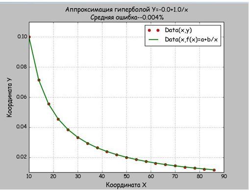
Мы брали данные из функции равносторонней гиперболы, поэтому и получили a=0,b=10 и абсолютную погрешность в 0,004%. Значить функция mnkGP(x,y) работает правильно и её можно вставлять в прикладную программу

Аппроксимация для степенных функций

Для этого в Python есть модуль scipy, но он не поддерживает отрицательную степень d полинома. Рассмотрим код реализации аппроксимации данных полиномом.

#!/usr/bin/python
# coding: utf8
import scipy as sp
import matplotlib.pyplot as plt
def mnkGP(x,y):
              d=2 # степень полинома
              fp, residuals, rank, sv, rcond = sp.polyfit(x, y, d, full=True) # Модель
              f = sp.poly1d(fp) # аппроксимирующая функция
              print('Коэффициент -- a %s  '%round(fp[0],4))
              print('Коэффициент-- b %s  '%round(fp[1],4))
              print('Коэффициент -- c %s  '%round(fp[2],4))
              y1=[fp[0]*x[i]**2+fp[1]*x[i]+fp[2] for i in range(0,len(x))] # значения функции a*x**2+b*x+c
              so=round(sum([abs(y[i]-y1[i]) for i in range(0,len(x))])/(len(x)*sum(y))*100,4) # средняя ошибка
              print('Average quadratic deviation '+str(so)) 
              fx = sp.linspace(x[0], x[-1] + 1, len(x)) # можно установить вместо len(x) большее число для интерполяции
              plt.plot(x, y, 'o', label='Original data', markersize=10)
              plt.plot(fx, f(fx), linewidth=2)
              plt.grid(True)
              plt.show()

x=[10, 14, 18, 22, 26, 30, 34, 38, 42, 46, 50, 54, 58, 62, 66, 70, 74, 78, 82, 86] 
y=[0.1, 0.0714, 0.0556, 0.0455, 0.0385, 0.0333, 0.0294, 0.0263, 0.0238, 0.0217,
   0.02, 0.0185, 0.0172, 0.0161, 0.0152, 0.0143, 0.0135, 0.0128, 0.0122,
   0.0116] # данные для проверки по функции y=1/x
mnkGP(x,y)

Результат

Как следует из графика, при аппроксимации параболой данных изменяющихся по гиперболе средняя ошибка возрастает, а свободный член квадратного уравнения обращается в ноль.

Полученные функции будут применены для анализа Законов Зипфа (Ципфа), но это будет сделано уже в следующей статье.

Ссылки:

1. Законы Зипфа (Ципфа) tpl-it.wikispaces.com/Законы+Зипфа+%28Ципфа%29
2. Закон Ципфа это. dic.academic.ru/dic.nsf/ruwiki/24105
3. Законы Зипфа. wiki.webimho.ru/законы-зипфа
4. Лекция 5. Аппроксимация функций по методу наименьших квадратов. mvm-math.narod.ru/Lec_PM5.pdf
5. Средняя ошибка аппроксимации. math.semestr.ru/corel/zadacha.php

The mean squared error is a common way to measure the prediction accuracy of a model. In this tutorial, you’ll learn how to calculate the mean squared error in Python. You’ll start off by learning what the mean squared error represents. Then you’ll learn how to do this using Scikit-Learn (sklean), Numpy, as well as from scratch.

What is the Mean Squared Error

The mean squared error measures the average of the squares of the errors. What this means, is that it returns the average of the sums of the square of each difference between the estimated value and the true value.

The MSE is always positive, though it can be 0 if the predictions are completely accurate. It incorporates the variance of the estimator (how widely spread the estimates are) and its bias (how different the estimated values are from their true values).

The formula looks like below:

Now that you have an understanding of how to calculate the MSE, let’s take a look at how it can be calculated using Python.

Interpreting the Mean Squared Error

The mean squared error is always 0 or positive. When a MSE is larger, this is an indication that the linear regression model doesn’t accurately predict the model.

An important piece to note is that the MSE is sensitive to outliers. This is because it calculates the average of every data point’s error. Because of this, a larger error on outliers will amplify the MSE.

There is no “target” value for the MSE. The MSE can, however, be a good indicator of how well a model fits your data. It can also give you an indicator of choosing one model over another.

Loading a Sample Pandas DataFrame

Let’s start off by loading a sample Pandas DataFrame. If you want to follow along with this tutorial line-by-line, simply copy the code below and paste it into your favorite code editor.

# Importing a sample Pandas DataFrame
import pandas as pd

df = pd.DataFrame.from_dict({
    'x': [1,2,3,4,5,6,7,8,9,10], 
    'y': [1,2,2,4,4,5,6,7,9,10]})

print(df.head())
#    x  y
# 0  1  1
# 1  2  2
# 2  3  2
# 3  4  4
# 4  5  4

You can see that the editor has loaded a DataFrame containing values for variables x and y. We can plot this data out, including the line of best fit using Seaborn’s .regplot() function:

# Plotting a line of best fit
import seaborn as sns
import matplotlib.pyplot as plt
sns.regplot(data=df, x='x', y='y', ci=None)
plt.ylim(bottom=0)
plt.xlim(left=0)
plt.show()

This returns the following visualization:

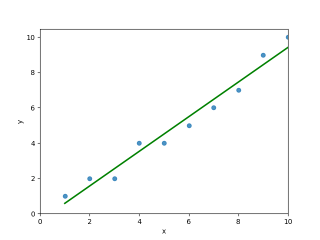
The mean squared error calculates the average of the sum of the squared differences between a data point and the line of best fit. By virtue of this, the lower a mean sqared error, the more better the line represents the relationship.

We can calculate this line of best using Scikit-Learn. You can learn about this in this in-depth tutorial on linear regression in sklearn. The code below predicts values for each x value using the linear model:

# Calculating prediction y values in sklearn
from sklearn.linear_model import LinearRegression

model = LinearRegression()
model.fit(df[['x']], df['y'])
y_2 = model.predict(df[['x']])
df['y_predicted'] = y_2
print(df.head())

# Returns:
#    x  y  y_predicted
# 0  1  1     0.581818
# 1  2  2     1.563636
# 2  3  2     2.545455
# 3  4  4     3.527273
# 4  5  4     4.509091

Calculating the Mean Squared Error with Scikit-Learn

The simplest way to calculate a mean squared error is to use Scikit-Learn (sklearn). The metrics module comes with a function, mean_squared_error() which allows you to pass in true and predicted values.

Let’s see how to calculate the MSE with sklearn:

# Calculating the MSE with sklearn
from sklearn.metrics import mean_squared_error
mse = mean_squared_error(df['y'], df['y_predicted'])
print(mse)

# Returns: 0.24727272727272714

This approach works very well when you’re already importing Scikit-Learn. That said, the function works easily on a Pandas DataFrame, as shown above.

In the next section, you’ll learn how to calculate the MSE with Numpy using a custom function.

Calculating the Mean Squared Error from Scratch using Numpy

Numpy itself doesn’t come with a function to calculate the mean squared error, but you can easily define a custom function to do this. We can make use of the subtract() function to subtract arrays element-wise.

# Definiting a custom function to calculate the MSE
import numpy as np

def mse(actual, predicted):
    actual = np.array(actual)
    predicted = np.array(predicted)
    differences = np.subtract(actual, predicted)
    squared_differences = np.square(differences)
    return squared_differences.mean()

print(mse(df['y'], df['y_predicted']))

# Returns: 0.24727272727272714

The code above is a bit verbose, but it shows how the function operates. We can cut down the code significantly, as shown below:

# A shorter version of the code above
import numpy as np

def mse(actual, predicted):
    return np.square(np.subtract(np.array(actual), np.array(predicted))).mean()

print(mse(df['y'], df['y_predicted']))

# Returns: 0.24727272727272714

Conclusion

In this tutorial, you learned what the mean squared error is and how it can be calculated using Python. First, you learned how to use Scikit-Learn’s mean_squared_error() function and then you built a custom function using Numpy.

The MSE is an important metric to use in evaluating the performance of your machine learning models. While Scikit-Learn abstracts the way in which the metric is calculated, understanding how it can be implemented from scratch can be a helpful tool.

Additional Resources

To learn more about related topics, check out the tutorials below:

• Pandas Variance: Calculating Variance of a Pandas Dataframe Column
• Calculate the Pearson Correlation Coefficient in Python
• How to Calculate a Z-Score in Python (4 Ways)
• Official Documentation from Scikit-Learn

How to Calculate Mean Squared Error in Python

The mean squared error is a common way to measure the prediction accuracy of a model. In this tutorial, you’ll learn how to calculate the mean squared error in Python. You’ll start off by learning what the mean squared error represents. Then you’ll learn how to do this using Scikit-Learn (sklean), Numpy, as well as from scratch.

What is the Mean Squared Error

The mean squared error measures the average of the squares of the errors. What this means, is that it returns the average of the sums of the square of each difference between the estimated value and the true value.

The MSE is always positive, though it can be 0 if the predictions are completely accurate. It incorporates the variance of the estimator (how widely spread the estimates are) and its bias (how different the estimated values are from their true values).

The formula looks like below:

An important piece to note is that the MSE is sensitive to outliers. This is because it calculates the average of every data point’s error. Because of this, a larger error on outliers will amplify the MSE.

There is no “target” value for the MSE. The MSE can, however, be a good indicator of how well a model fits your data. It can also give you an indicator of choosing one model over another.

Loading a Sample Pandas DataFrame

Let’s start off by loading a sample Pandas DataFrame. If you want to follow along with this tutorial line-by-line, simply copy the code below and paste it into your favorite code editor.

# Importing a sample Pandas DataFrame import pandas as pd df = pd.DataFrame.from_dict(< 'x': [1,2,3,4,5,6,7,8,9,10], 'y': [1,2,2,4,4,5,6,7,9,10]>) print(df.head()) # x y # 0 1 1 # 1 2 2 # 2 3 2 # 3 4 4 # 4 5 4

You can see that the editor has loaded a DataFrame containing values for variables x and y . We can plot this data out, including the line of best fit using Seaborn’s .regplot() function:

# Plotting a line of best fit import seaborn as sns import matplotlib.pyplot as plt sns.regplot(data=df, x='x', y='y', ci=None) plt.ylim(bottom=0) plt.xlim(left=0) plt.show()

This returns the following visualization:

The mean squared error calculates the average of the sum of the squared differences between a data point and the line of best fit. By virtue of this, the lower a mean sqared error, the more better the line represents the relationship.

We can calculate this line of best using Scikit-Learn. You can learn about this in this in-depth tutorial on linear regression in sklearn. The code below predicts values for each x value using the linear model:

# Calculating prediction y values in sklearn from sklearn.linear_model import LinearRegression model = LinearRegression() model.fit(df[['x']], df['y']) y_2 = model.predict(df[['x']]) df['y_predicted'] = y_2 print(df.head()) # Returns: # x y y_predicted # 0 1 1 0.581818 # 1 2 2 1.563636 # 2 3 2 2.545455 # 3 4 4 3.527273 # 4 5 4 4.509091

Calculating the Mean Squared Error with Scikit-Learn

The simplest way to calculate a mean squared error is to use Scikit-Learn (sklearn). The metrics module comes with a function, mean_squared_error() which allows you to pass in true and predicted values.

Let’s see how to calculate the MSE with sklearn:

# Calculating the MSE with sklearn from sklearn.metrics import mean_squared_error mse = mean_squared_error(df['y'], df['y_predicted']) print(mse) # Returns: 0.24727272727272714

This approach works very well when you’re already importing Scikit-Learn. That said, the function works easily on a Pandas DataFrame, as shown above.

In the next section, you’ll learn how to calculate the MSE with Numpy using a custom function.

Calculating the Mean Squared Error from Scratch using Numpy

Numpy itself doesn’t come with a function to calculate the mean squared error, but you can easily define a custom function to do this. We can make use of the subtract() function to subtract arrays element-wise.

# Definiting a custom function to calculate the MSE import numpy as np def mse(actual, predicted): actual = np.array(actual) predicted = np.array(predicted) differences = np.subtract(actual, predicted) squared_differences = np.square(differences) return squared_differences.mean() print(mse(df['y'], df['y_predicted'])) # Returns: 0.24727272727272714

The code above is a bit verbose, but it shows how the function operates. We can cut down the code significantly, as shown below:

# A shorter version of the code above import numpy as np def mse(actual, predicted): return np.square(np.subtract(np.array(actual), np.array(predicted))).mean() print(mse(df['y'], df['y_predicted'])) # Returns: 0.24727272727272714

Conclusion

In this tutorial, you learned what the mean squared error is and how it can be calculated using Python. First, you learned how to use Scikit-Learn’s mean_squared_error() function and then you built a custom function using Numpy.

The MSE is an important metric to use in evaluating the performance of your machine learning models. While Scikit-Learn abstracts the way in which the metric is calculated, understanding how it can be implemented from scratch can be a helpful tool.

Additional Resources

To learn more about related topics, check out the tutorials below:

Источник

Как рассчитать среднюю абсолютную ошибку в Python

В статистике средняя абсолютная ошибка (MAE) — это способ измерения точности данной модели. Он рассчитывается как:

• Σ: греческий символ, означающий «сумма».
• y i : Наблюдаемое значение для i -го наблюдения
• x i : Прогнозируемое значение для i -го наблюдения
• n: общее количество наблюдений

Мы можем легко вычислить среднюю абсолютную ошибку в Python, используя функцию mean_absolute_error() из Scikit-learn.

В этом руководстве представлен пример использования этой функции на практике.

Пример: вычисление средней абсолютной ошибки в Python

Предположим, у нас есть следующие массивы фактических значений и прогнозируемых значений в Python:

actual = [12, 13, 14, 15, 15, 22, 27] pred = [11, 13, 14, 14, 15, 16, 18] 

Следующий код показывает, как вычислить среднюю абсолютную ошибку для этой модели:

from sklearn. metrics import mean_absolute_error as mae #calculate MAE mae(actual, pred) 2.4285714285714284 

Средняя абсолютная ошибка (MAE) оказывается равной 2,42857 .

Это говорит нам о том, что средняя разница между фактическим значением данных и значением, предсказанным моделью, составляет 2,42857.

Мы можем сравнить эту MAE с MAE, полученной с помощью других моделей прогнозирования, чтобы увидеть, какие модели работают лучше всего.

Чем ниже MAE для данной модели, тем точнее модель способна предсказать фактические значения.

Примечание.Массив фактических значений и массив прогнозируемых значений должны иметь одинаковую длину, чтобы эта функция работала правильно.

Источник