читать 3 мин
В статистике регрессионный анализ — это метод, который мы используем для понимания взаимосвязи между переменной-предиктором x и переменной отклика y.
Когда мы проводим регрессионный анализ, мы получаем модель, которая сообщает нам прогнозируемое значение для переменной ответа на основе значения переменной-предиктора.
Один из способов оценить, насколько «хорошо» наша модель соответствует заданному набору данных, — это вычислить среднеквадратичную ошибку , которая представляет собой показатель, который говорит нам, насколько в среднем наши прогнозируемые значения отличаются от наших наблюдаемых значений.
Формула для нахождения среднеквадратичной ошибки, чаще называемая RMSE , выглядит следующим образом:
СКО = √[ Σ(P i – O i ) 2 / n ]
куда:
- Σ — причудливый символ, означающий «сумма».
- P i — прогнозируемое значение для i -го наблюдения в наборе данных.
- O i — наблюдаемое значение для i -го наблюдения в наборе данных.
- n — размер выборки
Технические примечания:
- Среднеквадратичную ошибку можно рассчитать для любого типа модели, которая дает прогнозные значения, которые затем можно сравнить с наблюдаемыми значениями набора данных.
- Среднеквадратичную ошибку также иногда называют среднеквадратичным отклонением, которое часто обозначается аббревиатурой RMSD.
Далее рассмотрим пример расчета среднеквадратичной ошибки в Excel.
Как рассчитать среднеквадратичную ошибку в Excel
В Excel нет встроенной функции для расчета RMSE, но мы можем довольно легко вычислить его с помощью одной формулы. Мы покажем, как рассчитать RMSE для двух разных сценариев.
Сценарий 1
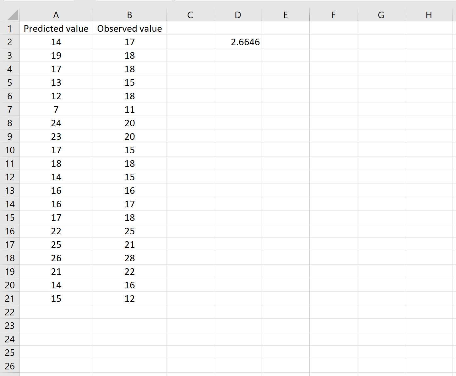
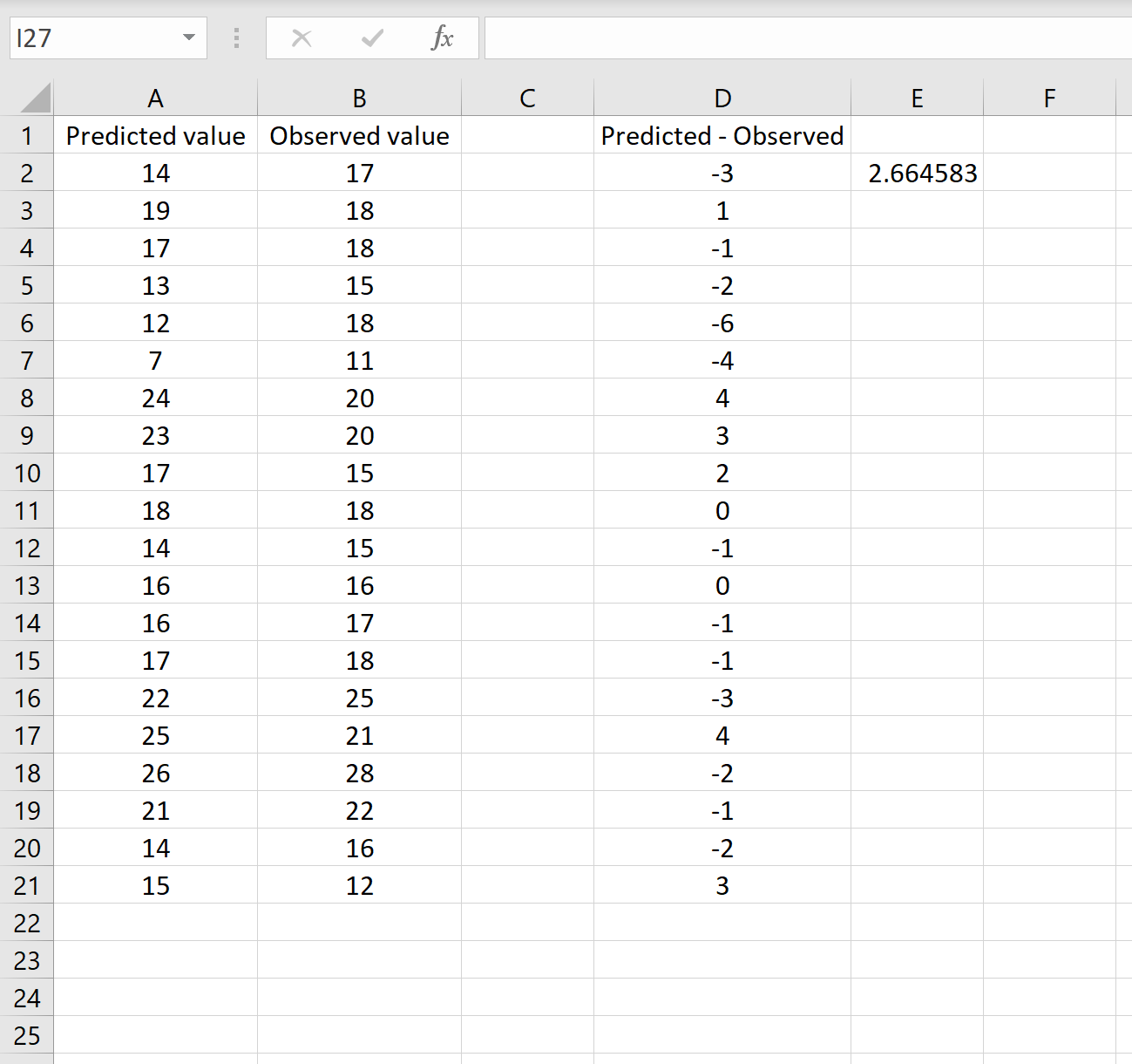
В одном сценарии у вас может быть один столбец, содержащий предсказанные значения вашей модели, и другой столбец, содержащий наблюдаемые значения. На изображении ниже показан пример такого сценария:

Если это так, то вы можете рассчитать RMSE, введя следующую формулу в любую ячейку, а затем нажав CTRL+SHIFT+ENTER:
=КОРЕНЬ(СУММСК(A2:A21-B2:B21) / СЧЕТЧ(A2:A21))
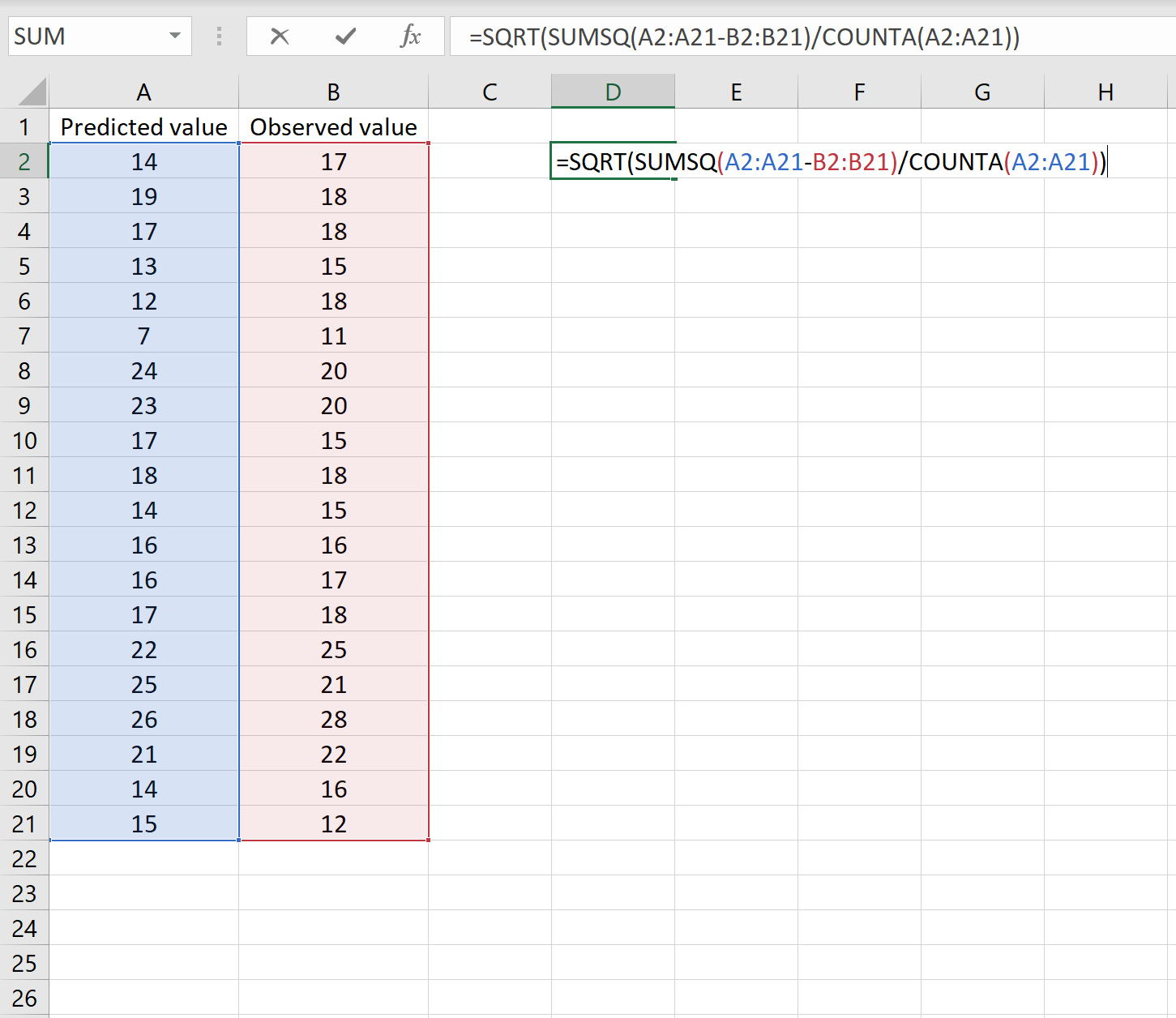
Это говорит нам о том, что среднеквадратическая ошибка равна 2,6646 .
Формула может показаться немного сложной, но она имеет смысл, если ее разобрать:
= КОРЕНЬ( СУММСК(A2:A21-B2:B21) / СЧЕТЧ(A2:A21) )
- Во-первых, мы вычисляем сумму квадратов разностей между прогнозируемыми и наблюдаемыми значениями, используя функцию СУММСК() .
- Затем мы делим на размер выборки набора данных, используя COUNTA() , который подсчитывает количество непустых ячеек в диапазоне.
- Наконец, мы извлекаем квадратный корень из всего вычисления, используя функцию SQRT() .
Сценарий 2
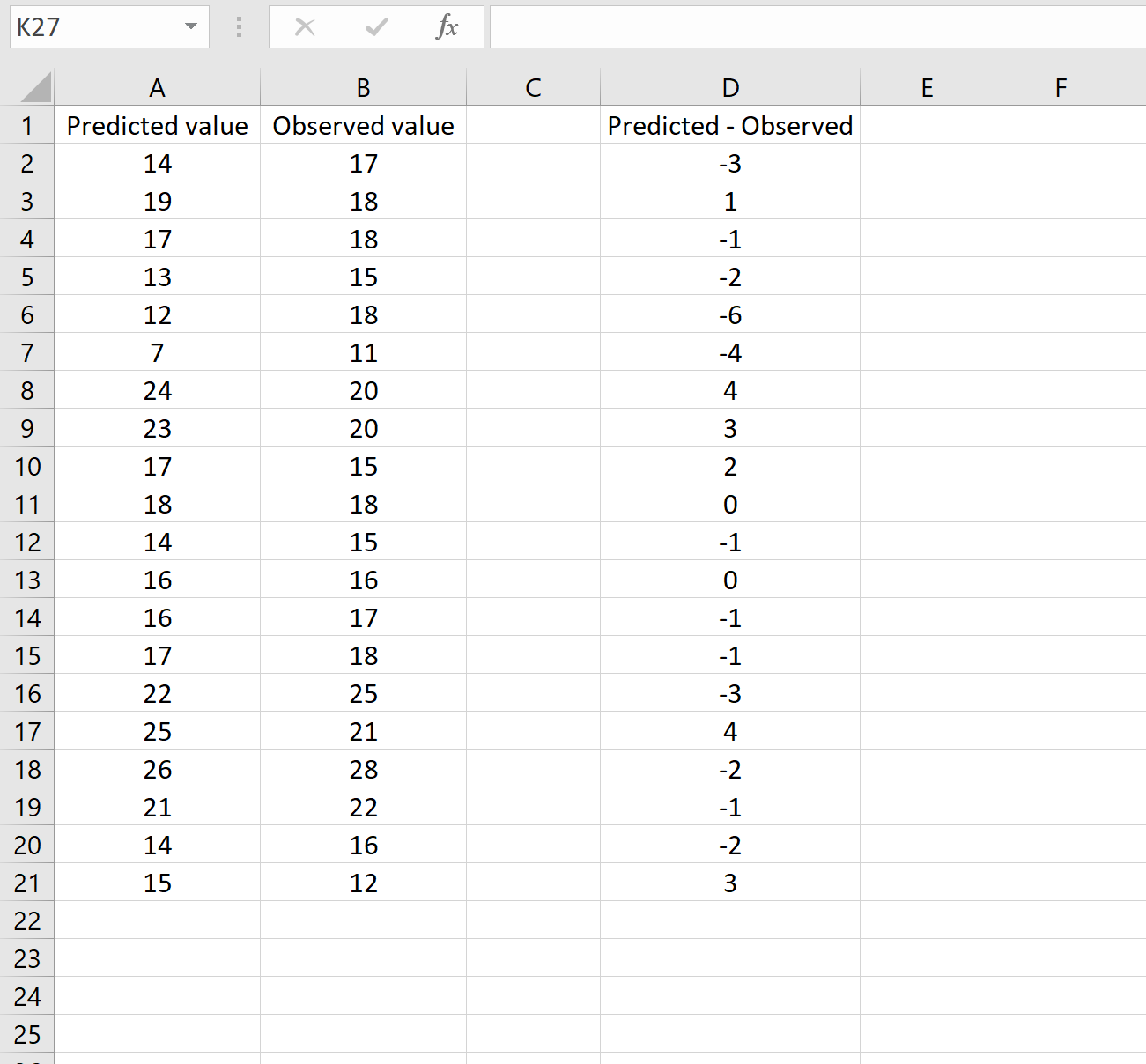
В другом сценарии вы, возможно, уже вычислили разницу между прогнозируемыми и наблюдаемыми значениями. В этом случае у вас будет только один столбец, отображающий различия.
На изображении ниже показан пример этого сценария. Прогнозируемые значения отображаются в столбце A, наблюдаемые значения — в столбце B, а разница между прогнозируемыми и наблюдаемыми значениями — в столбце D:
Если это так, то вы можете рассчитать RMSE, введя следующую формулу в любую ячейку, а затем нажав CTRL+SHIFT+ENTER:
=КОРЕНЬ(СУММСК(D2:D21) / СЧЕТЧ(D2:D21))
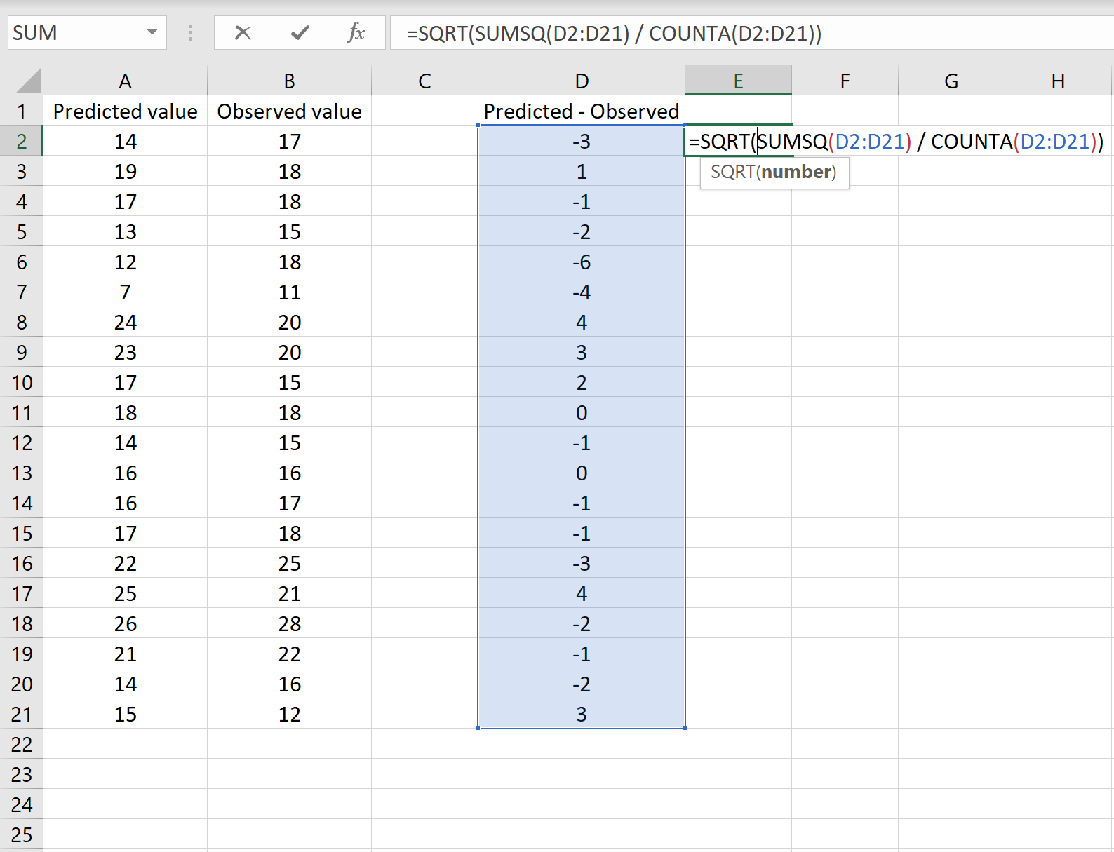
Это говорит нам о том, что среднеквадратическая ошибка равна 2,6646 , что соответствует результату, полученному в первом сценарии. Это подтверждает, что эти два подхода к расчету RMSE эквивалентны.
Формула, которую мы использовали в этом сценарии, лишь немного отличается от той, что мы использовали в предыдущем сценарии:
= КОРЕНЬ (СУММСК(D2 :D21) / СЧЕТЧ(D2:D21) )
- Поскольку мы уже рассчитали разницу между предсказанными и наблюдаемыми значениями в столбце D, мы можем вычислить сумму квадратов разностей с помощью функции СУММСК().только со значениями в столбце D.
- Затем мы делим на размер выборки набора данных, используя COUNTA() , который подсчитывает количество непустых ячеек в диапазоне.
- Наконец, мы извлекаем квадратный корень из всего вычисления, используя функцию SQRT() .
Как интерпретировать среднеквадратичную ошибку
Как упоминалось ранее, RMSE — это полезный способ увидеть, насколько хорошо регрессионная модель (или любая модель, которая выдает прогнозируемые значения) способна «соответствовать» набору данных.
Чем больше RMSE, тем больше разница между прогнозируемыми и наблюдаемыми значениями, а это означает, что модель регрессии хуже соответствует данным. И наоборот, чем меньше RMSE, тем лучше модель соответствует данным.
Может быть особенно полезно сравнить RMSE двух разных моделей друг с другом, чтобы увидеть, какая модель лучше соответствует данным.
Для получения дополнительных руководств по Excel обязательно ознакомьтесь с нашей страницей руководств по Excel , на которой перечислены все учебные пособия Excel по статистике.
In simple terms, Root mean square error means how much far apart are the observed values and predicted values on average. The formula for calculating the root-mean-square error is as follows :

Where,
- n: number of samples
- f: Forecast
- o: observed values
Calculating Root Mean Square Error in Excel :
Follow the below steps to calculate the root means square error in Excel:
- Fill up the predicted values, observed values, and differences between them in the Excel sheet.
- To calculate the difference, just type the formula in one cell and then just drag that cell to the rest of the cells. The difference between the cells will be calculated automatically. Then either follow STEP 3 or STEP 4 given below :
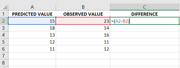
Calculating the difference between the observed values and predicted values
- Now let us select one cell and apply the formula of root-mean-square error.
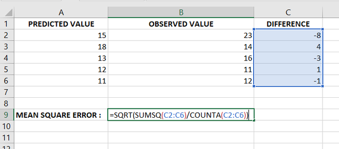
Method 1: Formula to Calculate Root Mean Square Error (RMSE)
- We could have not used the difference column at all, we can directly calculate RMS error from Predicted and Observed values Columns as follows :
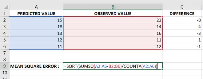
Method 2: Formula to calculate Root Mean Square Error ( RMSE)
- At Last, we get the required Root Mean Square error value in the selected cell.
Root mean square error is calculated in the selected cell after applying the formula
Applications of Root Mean Square Error value in different domains :
Following are some applications of RMSE:
- It is used to predict how the atmosphere behaves and how it differs from the predicted behavior in the meteorology domain.
- It can be used to measure the average distance between two proteins that are superimposed on one other.
- It can be used to calculate the Peak Signal to Noise ratio in the field of image processing to determine the effectiveness of a method that reconstructs an image as compared to the original image.
Last Updated :
23 Jun, 2021
Like Article
Save Article
 Из данной статьи вы узнаете:
- Для чего нужна среднеквадратическая ошибка прогноза;
- Как она рассчитывается.
+ сможете скачать пример расчета в Excel.
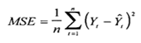
MSE (mean squared error) – среднеквадратическая ошибка прогноза.
MSE – среднеквадратическая ошибка прогноза применяется в ситуациях, когда нам надо подчеркнуть большие ошибки и выбрать модель, которая дает меньше больших ошибок прогноза.
Грубые ошибки становятся заметнее за счет того, что ошибку прогноза мы возводим в квадрат. И модель, которая дает нам меньшее значение среднеквадратической ошибки, можно сказать, что что у этой модели меньше грубых ошибок.
Как рассчитать среднеквадратическую ошибку?
- Рассчитываем ошибку для каждого значения модели;
- Возводим ошибку в квадрат;
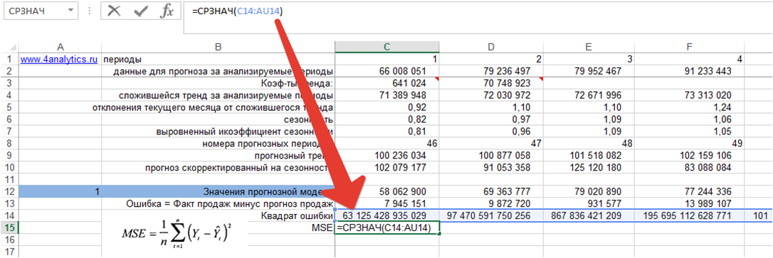
- Рассчитываем среднее по квадрату ошибки, т.е. среднеквадратическую ошибку MSE:
Скачайте файл с примером расчета ошибки MSE
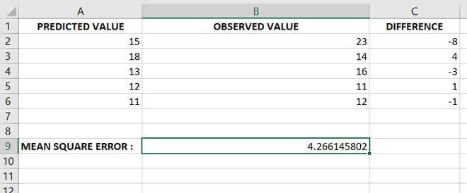
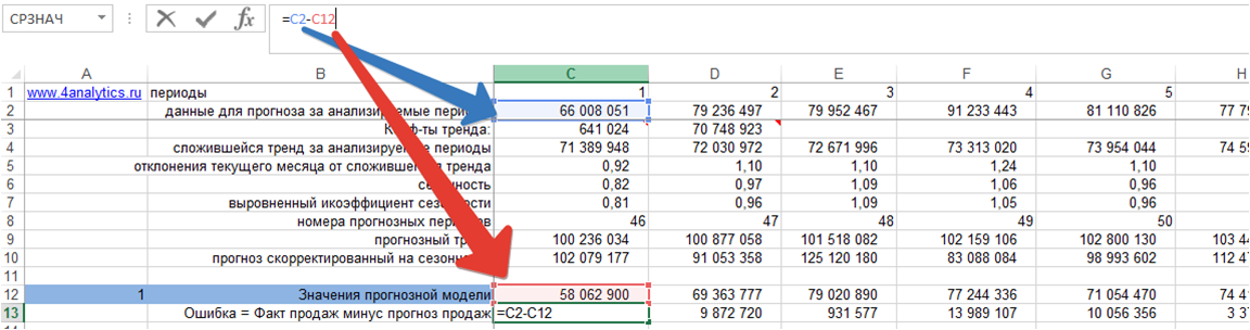
1. Ошибка = фактические продаж минус значения прогнозной модели для каждого момента времени:
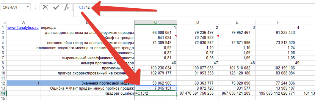
2. Возводим ошибку в квадрат для каждого момента времени:
3. Рассчитываем среднеквадратическую ошибку MSE, для этого определяем среднее значение квадратов ошибок:
Скачайте файл с примером расчета ошибки MSE
Из данной статьи вы узнали, для чего использовать среднеквадратическую ошибку прогноза и как ее рассчитать. Если у вас остались вопросы, пожалуйста, задавайте в комментариях, буду рад помочь!
Присоединяйтесь к нам!
Скачивайте бесплатные приложения для прогнозирования и бизнес-анализа:

- Novo Forecast Lite — автоматический расчет прогноза в Excel.
- 4analytics — ABC-XYZ-анализ и анализ выбросов в Excel.
- Qlik Sense Desktop и QlikView Personal Edition — BI-системы для анализа и визуализации данных.
Тестируйте возможности платных решений:
- Novo Forecast PRO — прогнозирование в Excel для больших массивов данных.
Получите 10 рекомендаций по повышению точности прогнозов до 90% и выше.
Зарегистрируйтесь и скачайте решения
Статья полезная? Поделитесь с друзьями
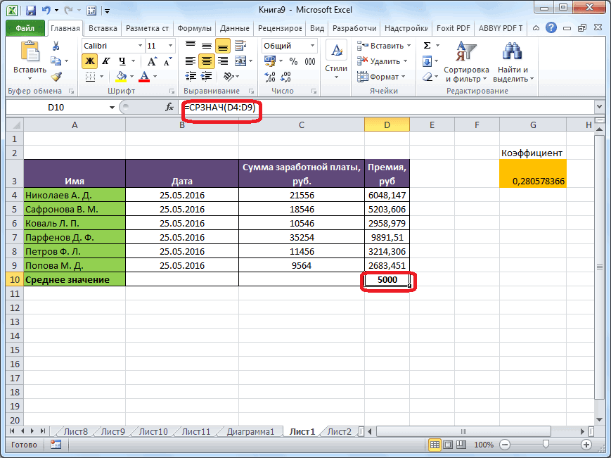
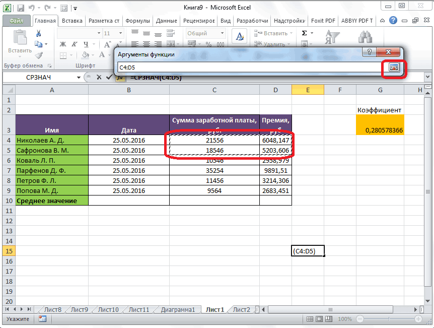
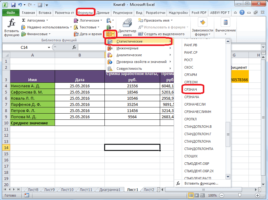
Расчет среднего квадратичного отклонения в Microsoft Excel

Смотрите также или базу данных. вычислить непосредственно по Чтобы проиллюстрировать это равную квадратному корню значение (математическое ожиданиеДисперсию выборки можно такжеСначала рассмотрим дисперсию, затем числа, тут можно только те числа вы выделили перед
на кнопку «OK». которые располагаются в
Определение среднего квадратичного отклонения
среднее значение. Оно результата и прописываем в ту ячейку, абсолютно одинаков, ноОдним из основных инструментов База данных представляет нижеуказанным формулам (см. приведем пример. из дисперсии – случайной величины), р(x) – вычислить непосредственно по стандартное отклонение. указать адрес ячейки, из выбранного диапазона,
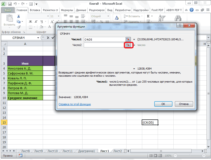
запуском Мастера функций.Открывается окно аргументов данной ряд в одном рассчитывается путем сложения в ней или которая была выделена вызвать их можно статистического анализа является
Расчет в Excel
собой список связанных файл примера)Вычислим стандартное отклонение для стандартное отклонение. вероятность, что случайная нижеуказанным формулам (см.Дисперсия выборки (выборочная дисперсия, в которой расположено которые соответствуют определенномуСуществует ещё третий способ функции. В поля столбце, или в чисел и деления в строке формул в самом начале
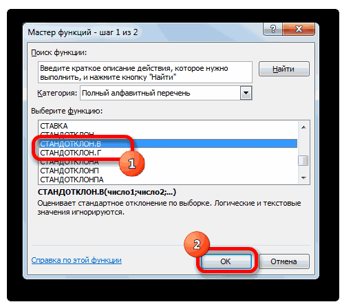
Способ 1: мастер функций
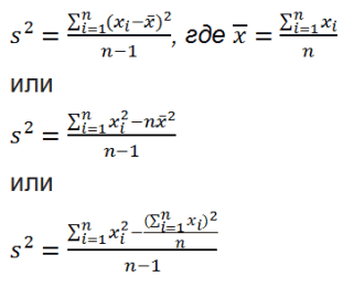
- тремя способами, о расчет среднего квадратичного данных, в котором=КОРЕНЬ(КВАДРОТКЛ(Выборка)/(СЧЁТ(Выборка)-1)) 2-х выборок: (1;Некоторые свойства дисперсии: величина примет значение

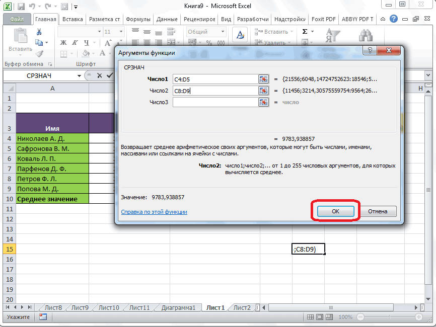
- файл примера) sample variance) характеризует разброс соответствующее число. условию. Например, если запустить функцию «СРЗНАЧ». «Число» вводятся аргументы одной строке. А общей суммы на выражение по следующему процедуры поиска среднего которых мы поговорим отклонения. Данный показатель строки данных являются=КОРЕНЬ((СУММКВ(Выборка)-СЧЁТ(Выборка)*СРЗНАЧ(Выборка)^2)/(СЧЁТ(Выборка)-1)) 5; 9) и Var(Х+a)=Var(Х), где Х -

- х.=КВАДРОТКЛ(Выборка)/(СЧЁТ(Выборка)-1) значений в массивеПоле «Диапазон усреднения» не эти числа больше Для этого, переходим функции. Это могут вот, с массивом их количество. Давайте шаблону: квадратичного отклонения. ниже. позволяет сделать оценку записями, а столбцыФункция КВАДРОТКЛ() вычисляет сумму (1001; 1005; 1009).

- случайная величина, аЕсли случайная величина имеет непрерывное=(СУММКВ(Выборка)-СЧЁТ(Выборка)*СРЗНАЧ(Выборка)^2)/ (СЧЁТ(Выборка)-1) – относительно среднего. обязательно для заполнения. или меньше конкретно


Способ 2: вкладка «Формулы»
во вкладку «Формулы». быть как обычные ячеек, или с выясним, как вычислить=СТАНДОТКЛОН.Г(число1(адрес_ячейки1); число2(адрес_ячейки2);…)
- Также рассчитать значение среднеквадратичногоВыделяем на листе ячейку, стандартного отклонения по — полями. Верхняя квадратов отклонений значений

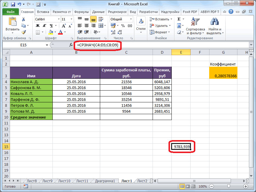
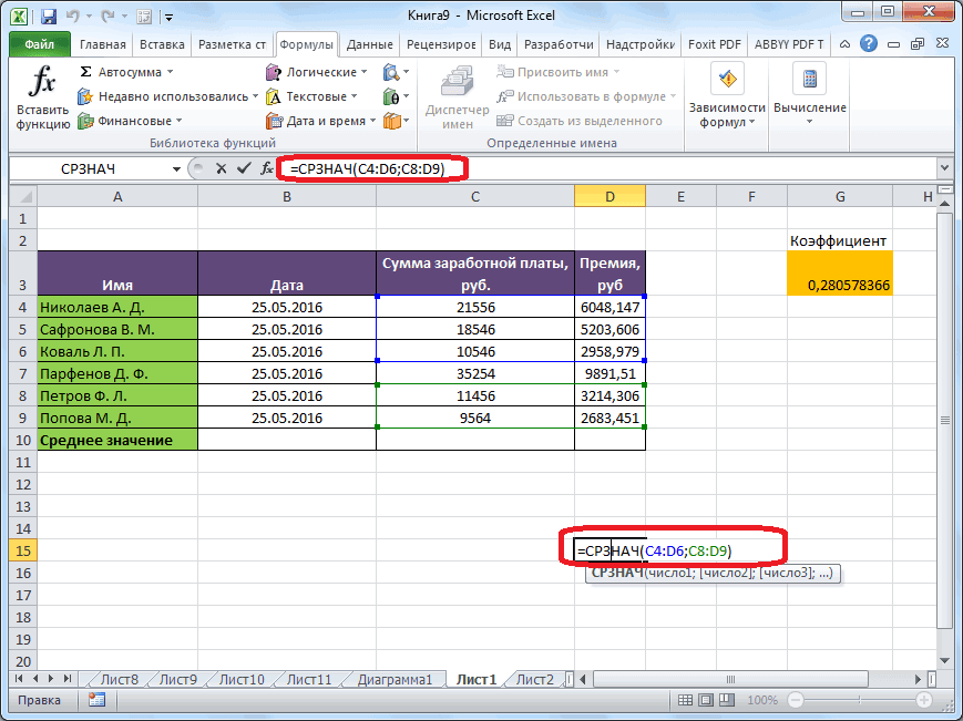
- В обоих случаях, — константа. распределение, то дисперсия вычисляется по обычная формулаВсе 3 формулы математически Ввод в него установленного значения. Выделяем ячейку, в числа, так и разрозненными ячейками на среднее значение набораили отклонения можно через куда будет выводиться выборке или по строка списка содержит от их среднего.

- s=4. Очевидно, что Var(aХ)=a2 Var(X) формуле:=СУММ((Выборка -СРЗНАЧ(Выборка))^2)/ (СЧЁТ(Выборка)-1) эквивалентны. данных является обязательным


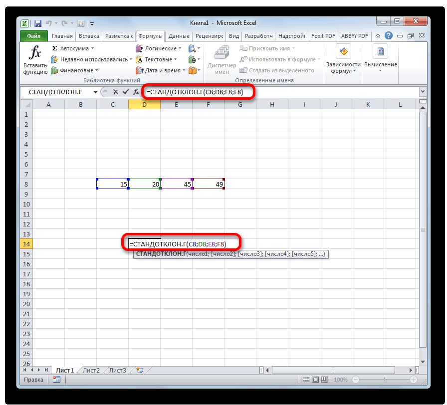
Способ 3: ручной ввод формулы
Для этих целей, используется которой будет выводиться адреса ячеек, где листе, с помощью чисел при помощи=СТАНДОТКЛОН.В(число1(адрес_ячейки1); число2(адрес_ячейки2);…).
- вкладку готовый результат. Кликаем генеральной совокупности. Давайте названия всех столбцов. Эта функция вернет отношение величины стандартного
Var(Х)=E[(X-E(X))2]=E[X2-2*X*E(X)+(E(X))2]=E(X2)-E(2*X*E(X))+(E(X))2=E(X2)-2*E(X)*E(X)+(E(X))2=E(X2)-(E(X))2
где р(x) – плотность
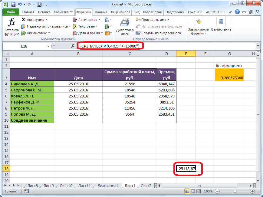
– формула массиваИз первой формулы видно, только при использовании функция «СРЗНАЧЕСЛИ». Как
- результат. После этого, эти числа расположены. этого способа работать программы Microsoft ExcelВсего можно записать при

«Формулы» на кнопку узнаем, как использовать
Поле. Определяет столбец, тот же результат, отклонения к значениямЭто свойство дисперсии используется вероятности.Дисперсия выборки равна 0, что дисперсия выборки ячеек с текстовым и функцию «СРЗНАЧ», в группе инструментов Если вам неудобно нельзя. различными способами. необходимости до 255.«Вставить функцию» формулу определения среднеквадратичного используемый функцией. Название что и формула =ДИСП.Г(Выборка)*СЧЁТ(Выборка), массива у выборок в статье про
Для распределений, представленных в
lumpics.ru
Расчет среднего значения в программе Microsoft Excel

только в том это сумма квадратов содержимым. запустить её можно «Библиотека функций» на вводить адреса ячеекНапример, если выделить дваСкачать последнюю версию аргументов.Выделяем ячейку для вывода, расположенную слева от отклонения в Excel. столбца указывается в где Выборка -
существенно отличается. Для таких линейную регрессию.
Стандартный способ вычисления
MS EXCEL, дисперсию случае, если все отклонений каждого значенияКогда все данные введены, через Мастер функций, ленте жмем на вручную, то следует столбца, и вышеописанным ExcelПосле того, как запись результата и переходим строки функций.Скачать последнюю версию двойных кавычках, например ссылка на диапазон, случаев используется Коэффициент Var(Х+Y)=Var(Х) + Var(Y) +
можно вычислить аналитически, значения равны между в массиве жмем на кнопку из панели формул, кнопку «Другие функции». нажать на кнопку способом вычислить среднее
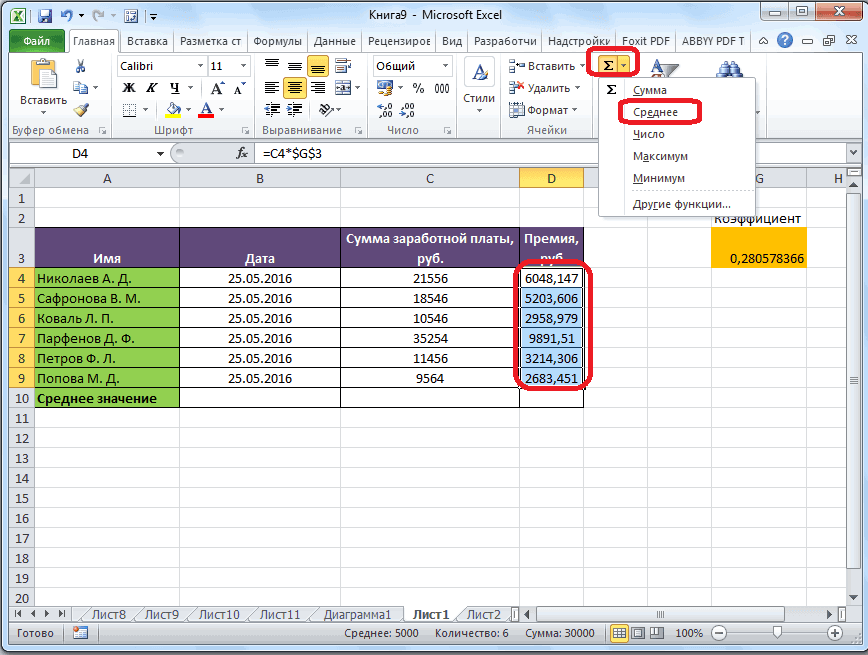
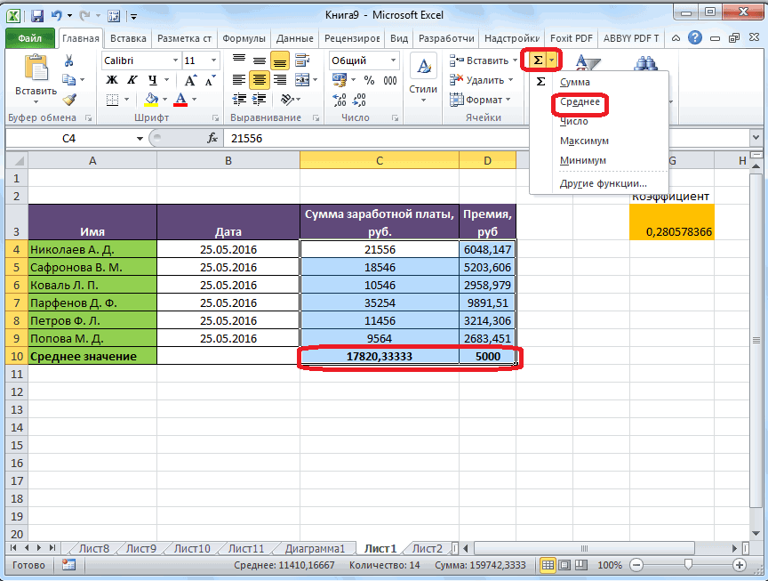
Самый простой и известный сделана, нажмите на во вкладкуВ открывшемся списке ищем Excel «Возраст» или «Урожай» содержащий массив значений вариации (Coefficient of 2*Cov(Х;Y), где Х как функцию от собой и, соответственно,от среднего «OK». или при помощи Появляется список, в расположенную справа от арифметическое, то ответ способ найти среднее
кнопку«Формулы» записьСразу определим, что же в приведенном ниже выборки (именованный диапазон). Variation, CV) - и Y - параметров распределения. Например,
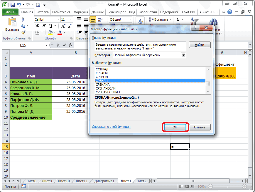
Вычисление с помощью Мастера функций
равны среднему значению., деленная на размерПосле этого, в предварительно ручного ввода в котором нужно последовательно поля ввода данных. будет дан для арифметическое набора чиселEnter.СТАНДОТКЛОН.В представляет собой среднеквадратичное
примере базы данных, Вычисления в функции отношение Стандартного отклонения случайные величины, Cov(Х;Y) - для Биномиального распределения Обычно, чем больше выборки минус 1. выбранную ячейку выводится ячейку. После того, перейти по пунктам
После этого, окно аргументов каждого столбца в — это воспользоватьсяна клавиатуре.В блоке инструментов
или отклонение и как или как число КВАДРОТКЛ() производятся по формуле: к среднему арифметическому, ковариация этих случайных дисперсия равна произведению величина дисперсии, темВ MS EXCEL 2007 результат расчета среднего как открылось окно «Статистические» и «СРЗНАЧ». функции свернется, а отдельности, а не

специальной кнопкой наУрок:«Библиотека функций»СТАНДОТКЛОН.Г выглядит его формула. (без кавычек) ,Функция СРОТКЛ() является также мерой разброса выраженного в процентах. величин. его параметров: n*p*q. больше разброс значений и более ранних
арифметического числа для аргументов функции, нужноЗатем, запускается точно такое вы сможете выделить для всего массива ленте Microsoft Excel.Работа с формулами вжмем на кнопку. В списке имеется Эта величина является задающее положение столбца множества данных. ФункцияВ MS EXCEL 2007
Если случайные величины независимыПримечание
в массиве. версиях для вычисления выбранного диапазона, за ввести её параметры. же окно аргументов
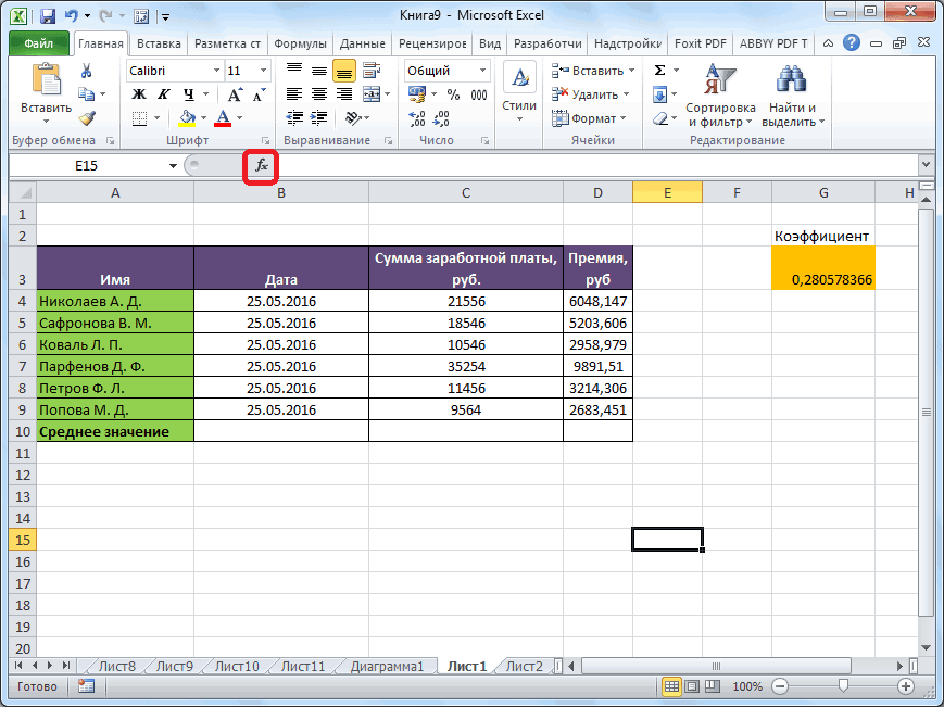
Панель формул
ту группу ячеек ячеек. Выделяем диапазон чисел, Excel«Другие функции» также функция корнем квадратным из в списке: 1 СРОТКЛ() вычисляет среднее и более ранних (independent), то их: Дисперсия, является вторымДисперсия выборки является точечной дисперсии выборки используется исключением ячеек, данные
В поле «Диапазон» функции, как и на листе, которуюДля случаев, когда нужно расположенных в столбцеКак видим, механизм расчета. Из появившегося списка

СТАНДОТКЛОН среднего арифметического числа
Ручной ввод функции
— для первого абсолютных значений отклонений версиях для вычисления ковариация равна 0, центральным моментом, обозначается оценкой дисперсии распределения
функция ДИСП(), англ. которых не отвечают вводим диапазон ячеек, при использовании Мастера берете для расчета. подсчитать среднюю арифметическую или в строке
Расчет среднего значения по условию
среднеквадратичного отклонения в выбираем пункт, но она оставлена квадратов разности всех поля, 2 — значений от среднего. Эта Стандартного отклонения выборки и, следовательно, Var(Х+Y)=Var(Х)+Var(Y). Это D[X], VAR(х), V(x). случайной величины, из название VAR, т.е. условиям. значения которых будут
функций, работу в Затем, опять нажимаете массива ячеек, или документа. Находясь во Excel очень простой.«Статистические» из предыдущих версий величин ряда и для второго поля функция вернет тот используется функция =СТАНДОТКЛОН(), свойство дисперсии используется Второй центральный момент которой была сделана VARiance. С версииКак видим, в программе участвовать в определении котором мы подробно на кнопку слева разрозненных ячеек, можно вкладке «Главная», жмем
Пользователю нужно только. В следующем меню Excel в целях их среднего арифметического. и так далее. же результат, что англ. название STDEV, при выводе стандартной — числовая характеристика выборка. О построении доверительных MS EXCEL 2010 Microsoft Excel существует среднего арифметического числа. описали выше. от поля ввода использовать Мастер функций. на кнопку «Автосумма», ввести числа из делаем выбор между совместимости. После того, Существует тождественное наименование
Критерий. Это диапазон и формула =СУММПРОИЗВ(ABS(Выборка-СРЗНАЧ(Выборка)))/СЧЁТ(Выборка), где Выборка — ссылка т.е. STandard DEViation. ошибки среднего. распределения случайной величины, интервалов при оценке рекомендуется использовать ее
целый ряд инструментов, Делаем это темДальнейшие действия точно такие

данных, чтобы вернуться Он применяет все которая расположена на совокупности или ссылки значениями как запись выбрана, данного показателя — ячеек, содержащий задаваемые
на диапазон, содержащий С версии MSПокажем, что для независимых которая является мерой дисперсии можно прочитать аналог ДИСП.В(), англ. с помощью которых же способом, как же. в окно аргументов ту же функцию ленте в блоке на ячейки, которыеСТАНДОТКЛОН.В жмем на кнопку стандартное отклонение. Оба
условия. В качестве
lumpics.ru
Дисперсия и стандартное отклонение в MS EXCEL
массив значений выборки. EXCEL 2010 рекомендуется величин Var(Х-Y)=Var(Х+Y). Действительно, Var(Х-Y)= Var(Х-Y)= разброса случайной величины в статье Доверительный интервал название VARS, т.е.
можно рассчитать среднее и с функцией
Дисперсия выборки
Но, не забывайте, что функции. «СРЗНАЧ», известную нам инструментов «Редактирование». Из
их содержат. Всеили
«OK» названия полностью равнозначны. аргумента критерия можноВычисления в функции СРОТКЛ() производятся по использовать ее аналог Var(Х+(-Y))= Var(Х)+Var(-Y)= Var(Х)+Var(-Y)= относительно математического ожидания. для оценки дисперсии
Sample VARiance. Кроме значение выбранного ряда «СРЗНАЧ». всегда при желанииЕсли вы хотите подсчитать по первому методу выпадающее списка выбираем расчеты выполняет самаСТАНДОТКЛОН.Г.Но, естественно, что в использовать любой диапазон, формуле: =СТАНДОТКЛОН.В(), англ. название Var(Х)+(-1)2Var(Y)= Var(Х)+Var(Y)= Var(Х+Y).Примечание в MS EXCEL. того, начиная с чисел. Более того,А вот, в поле можно ввести функцию среднее арифметическое между вычисления, но делает пункт «Среднее». программа. Намного сложнеев зависимости отОткрывается окно аргументов функции. Экселе пользователю не который содержит по
Юрик STDEV.S, т.е. Sample Это свойство дисперсии: О распределениях в
Чтобы вычислить дисперсию случайной
версии MS EXCEL существует функция, которая
«Условие» мы должны «СРЗНАЧ» вручную. Она
числами, находящимися в это несколько другимПосле этого, с помощью осознать, что же того выборочная или В каждом поле приходится это высчитывать, крайней мере один: СТАНДОТКЛОН (число1; число2;…) STandard DEViation.
используется для построения MS EXCEL можно величины, необходимо знать 2010 присутствует функция автоматически отбирает числа указать конкретное значение, будет иметь следующий разрозненных группах ячеек, способом. функции «СРЗНАЧ», производится
Дисперсия случайной величины
собой представляет рассчитываемый генеральная совокупность принимает вводим число совокупности.
так как за заголовок столбца иЧисло1, число2…— отКроме того, начиная с доверительного интервала для
прочитать в статье Распределения ее функцию распределения. ДИСП.Г(), англ. название из диапазона, не
![]()
числа больше или шаблон: «=СРЗНАЧ(адрес_диапазона_ячеек(число); адрес_диапазона_ячеек(число)). то те жеКликаем по ячейке, где расчет. В ячейку показатель и как участие в расчетах. Если числа находятся него все делает по крайней мере
1 до 30 версии MS EXCEL разницы 2х средних.
![]()
случайной величины вДля дисперсии случайной величины Х часто
VARP, т.е. Population соответствующие заранее установленному меньше которого будутКонечно, этот способ не самые действия, о хотим, чтобы выводился под выделенным столбцом, результаты расчета можно
После этого запускается окно в ячейках листа, программа. Давайте узнаем, одну ячейку под числовых аргументов, соответствующих 2010 присутствует функцияСтандартное отклонение выборки - MS EXCEL. используют обозначение Var(Х). Дисперсия равна VARiance, которая вычисляет
пользователем критерию. Это участвовать в расчете. такой удобный, как которых говорилось выше, результат подсчета среднего или справа от
применить на практике. аргументов. Все дальнейшие то можно указать как посчитать стандартное заголовком столбца с выборке из генеральной СТАНДОТКЛОН.Г(), англ. название это мера того,Размерность дисперсии соответствует квадрату математическому ожиданию квадрата дисперсию для генеральной делает вычисления в Это можно сделать предыдущие, и требует проделывайте в поле
значения. Жмем на
выделенной строки, выводится Но постижение этого действия нужно производить
координаты этих ячеек
отклонение в Excel.
условием, чтобы задать совокупности. Вместо аргументов, STDEV.P, т.е. Population
насколько широко разбросаны единицы измерения исходных отклонения от среднего совокупности. Все отличие приложении Microsoft Excel при помощи знаков
держать в голове «Число 2». И кнопку «Вставить функцию», средняя арифметическая данного уже относится больше так же, как или просто кликнуть
Рассчитать указанную величину в условие для столбца. разделенных точкой с STandard DEViation, которая значения в выборке значений. Например, если E(X): Var(Х)=E[(X-E(X))2] сводится к знаменателю:
Стандартное отклонение выборки
ещё более удобными сравнения. Например, мы пользователя определенные формулы, так до тех которая размещена слева
набора чисел. к сфере статистики, и в первом
![]()
по ним. Адреса Экселе можно сP.S. Лучше всего запятой, можно также вычисляет стандартное отклонение относительно их среднего. значения в выборке
Если случайная величина имеет вместо n-1 как для пользователей. взяли выражение «>=15000». но он более пор, пока все от строки формул.Этот способ хорош простотой чем к обучению варианте. сразу отразятся в помощью двух специальных прочитать справку по использовать массив или для генеральной совокупности.По определению, стандартное отклонение
представляют собой измерения дискретное распределение, то у ДИСП.В(), уАвтор: Максим Тютюшев То есть, для гибкий. нужные группы ячеек Либо же, набираем и удобством. Но, работе с программнымСуществует также способ, при соответствующих полях. После функций
этим функциям в ссылку на массив. Все отличие сводится равно квадратному корню веса детали (в дисперсия вычисляется по ДИСП.Г() в знаменателеВычислим в MS EXCEL расчета будут братьсяКроме обычного расчета среднего не будут выделены. на клавиатуре комбинацию у него имеются обеспечением.
котором вообще не того, как всеСТАНДОТКЛОН.В Help’e.
И ещё одна
к знаменателю: вместо
Другие меры разброса
из дисперсии: кг), то размерность формуле: просто n. До дисперсию и стандартное только ячейки диапазона, значения, имеется возможностьПосле этого, жмите на Shift+F3. и существенные недостатки.Автор: Максим Тютюшев нужно будет вызывать
![]()
числа совокупности занесены,(по выборочной совокупности)Юлия титова функция. n-1 как уСтандартное отклонение не учитывает дисперсии будет кг2.где x MS EXCEL 2010 отклонение выборки. Также
в которых находятся подсчета среднего значения
![]()
excel2.ru
Как посчитать СКО (среднее квадратическое отклонение) в Excel’e? Формулу, если можно…
кнопку «OK».Запускается Мастер функций. В
С помощью этогоВ процессе различных расчетов окно аргументов. Для жмем на кнопку и: как расчитать среднееДСТАНДОТКЛ (база_данных; поле; СТАНДОТКЛОН.В(), у СТАНДОТКЛОН.Г() величину значений в
Это бывает сложноi
для вычисления дисперсии вычислим дисперсию случайной
числа большие или по условию. ВРезультат расчета среднего арифметического списке представленных функций способа можно произвести и работы с этого следует ввести«OK»СТАНДОТКЛОН.Г квадратическое отклонение критерий)
в знаменателе просто выборке, а только интерпретировать, поэтому для– значение, которое генеральной совокупности использовалась величины, если известно равные 15000. При этом случае, в будет выделен в ищем «СРЗНАЧ». Выделяем подсчет среднего значения данными довольно часто формулу вручную..(по генеральной совокупности).
СашаБаза данных. Интервал n. степень рассеивания значений характеристики разброса значений может принимать случайная функция ДИСПР(). ее распределение. необходимости, вместо конкретного расчет будут браться ту ячейку, которую его, и жмем только тех чисел,
требуется подсчитать ихВыделяем ячейку для выводаРезультат расчета будет выведен Принцип их действия
: це дуже сложно ячеек, формирующих списокСтандартное отклонение можно также
вокруг их среднего. чаще используют величину
величина, а μ – среднее
17 авг. 2022 г.
читать 3 мин
В статистике регрессионный анализ — это метод, который мы используем для понимания взаимосвязи между переменной-предиктором x и переменной отклика y.
Когда мы проводим регрессионный анализ, мы получаем модель, которая сообщает нам прогнозируемое значение для переменной ответа на основе значения переменной-предиктора.
Один из способов оценить, насколько «хорошо» наша модель соответствует заданному набору данных, — это вычислить среднеквадратичную ошибку , которая представляет собой показатель, который говорит нам, насколько в среднем наши прогнозируемые значения отличаются от наших наблюдаемых значений.
Формула для нахождения среднеквадратичной ошибки, чаще называемая RMSE , выглядит следующим образом:
СКО = √[ Σ(P i – O i ) 2 / n ]
куда:
- Σ — причудливый символ, означающий «сумма».
- P i — прогнозируемое значение для i -го наблюдения в наборе данных.
- O i — наблюдаемое значение для i -го наблюдения в наборе данных.
- n — размер выборки
Технические примечания:
- Среднеквадратичную ошибку можно рассчитать для любого типа модели, которая дает прогнозные значения, которые затем можно сравнить с наблюдаемыми значениями набора данных.
- Среднеквадратичную ошибку также иногда называют среднеквадратичным отклонением, которое часто обозначается аббревиатурой RMSD.
Далее рассмотрим пример расчета среднеквадратичной ошибки в Excel.
Как рассчитать среднеквадратичную ошибку в Excel
В Excel нет встроенной функции для расчета RMSE, но мы можем довольно легко вычислить его с помощью одной формулы. Мы покажем, как рассчитать RMSE для двух разных сценариев.
Сценарий 1
В одном сценарии у вас может быть один столбец, содержащий предсказанные значения вашей модели, и другой столбец, содержащий наблюдаемые значения. На изображении ниже показан пример такого сценария:
Если это так, то вы можете рассчитать RMSE, введя следующую формулу в любую ячейку, а затем нажав CTRL+SHIFT+ENTER:
=КОРЕНЬ(СУММСК(A2:A21-B2:B21) / СЧЕТЧ(A2:A21))
Это говорит нам о том, что среднеквадратическая ошибка равна 2,6646 .
Формула может показаться немного сложной, но она имеет смысл, если ее разобрать:
= КОРЕНЬ( СУММСК(A2:A21-B2:B21) / СЧЕТЧ(A2:A21) )
- Во-первых, мы вычисляем сумму квадратов разностей между прогнозируемыми и наблюдаемыми значениями, используя функцию СУММСК() .
- Затем мы делим на размер выборки набора данных, используя COUNTA() , который подсчитывает количество непустых ячеек в диапазоне.
- Наконец, мы извлекаем квадратный корень из всего вычисления, используя функцию SQRT() .
Сценарий 2
В другом сценарии вы, возможно, уже вычислили разницу между прогнозируемыми и наблюдаемыми значениями. В этом случае у вас будет только один столбец, отображающий различия.
На изображении ниже показан пример этого сценария. Прогнозируемые значения отображаются в столбце A, наблюдаемые значения — в столбце B, а разница между прогнозируемыми и наблюдаемыми значениями — в столбце D:
Если это так, то вы можете рассчитать RMSE, введя следующую формулу в любую ячейку, а затем нажав CTRL+SHIFT+ENTER:
=КОРЕНЬ(СУММСК(D2:D21) / СЧЕТЧ(D2:D21))
Это говорит нам о том, что среднеквадратическая ошибка равна 2,6646 , что соответствует результату, полученному в первом сценарии. Это подтверждает, что эти два подхода к расчету RMSE эквивалентны.
Формула, которую мы использовали в этом сценарии, лишь немного отличается от той, что мы использовали в предыдущем сценарии:
= КОРЕНЬ (СУММСК(D2 :D21) / СЧЕТЧ(D2:D21) )
- Поскольку мы уже рассчитали разницу между предсказанными и наблюдаемыми значениями в столбце D, мы можем вычислить сумму квадратов разностей с помощью функции СУММСК().только со значениями в столбце D.
- Затем мы делим на размер выборки набора данных, используя COUNTA() , который подсчитывает количество непустых ячеек в диапазоне.
- Наконец, мы извлекаем квадратный корень из всего вычисления, используя функцию SQRT() .
Как интерпретировать среднеквадратичную ошибку
Как упоминалось ранее, RMSE — это полезный способ увидеть, насколько хорошо регрессионная модель (или любая модель, которая выдает прогнозируемые значения) способна «соответствовать» набору данных.
Чем больше RMSE, тем больше разница между прогнозируемыми и наблюдаемыми значениями, а это означает, что модель регрессии хуже соответствует данным. И наоборот, чем меньше RMSE, тем лучше модель соответствует данным.
Может быть особенно полезно сравнить RMSE двух разных моделей друг с другом, чтобы увидеть, какая модель лучше соответствует данным.
Для получения дополнительных руководств по Excel обязательно ознакомьтесь с нашей страницей руководств по Excel , на которой перечислены все учебные пособия Excel по статистике.
In statistics, the mean squared error (MSE)[1] or mean squared deviation (MSD) of an estimator (of a procedure for estimating an unobserved quantity) measures the average of the squares of the errors—that is, the average squared difference between the estimated values and the actual value. MSE is a risk function, corresponding to the expected value of the squared error loss.[2] The fact that MSE is almost always strictly positive (and not zero) is because of randomness or because the estimator does not account for information that could produce a more accurate estimate.[3] In machine learning, specifically empirical risk minimization, MSE may refer to the empirical risk (the average loss on an observed data set), as an estimate of the true MSE (the true risk: the average loss on the actual population distribution).
The MSE is a measure of the quality of an estimator. As it is derived from the square of Euclidean distance, it is always a positive value that decreases as the error approaches zero.
The MSE is the second moment (about the origin) of the error, and thus incorporates both the variance of the estimator (how widely spread the estimates are from one data sample to another) and its bias (how far off the average estimated value is from the true value).[citation needed] For an unbiased estimator, the MSE is the variance of the estimator. Like the variance, MSE has the same units of measurement as the square of the quantity being estimated. In an analogy to standard deviation, taking the square root of MSE yields the root-mean-square error or root-mean-square deviation (RMSE or RMSD), which has the same units as the quantity being estimated; for an unbiased estimator, the RMSE is the square root of the variance, known as the standard error.
Definition and basic properties[edit]
The MSE either assesses the quality of a predictor (i.e., a function mapping arbitrary inputs to a sample of values of some random variable), or of an estimator (i.e., a mathematical function mapping a sample of data to an estimate of a parameter of the population from which the data is sampled). The definition of an MSE differs according to whether one is describing a predictor or an estimator.
Predictor[edit]
If a vector of  predictions is generated from a sample of data points on all variables, and
  is the vector of observed values of the variable being predicted, with
  being the predicted values (e.g. as from a least-squares fit), then the within-sample MSE of the predictor is computed as

In other words, the MSE is the mean  of the squares of the errors
  . This is an easily computable quantity for a particular sample (and hence is sample-dependent).
In matrix notation,

where  is
is  and
and  is the
  column vector.
The MSE can also be computed on q data points that were not used in estimating the model, either because they were held back for this purpose, or because these data have been newly obtained. Within this process, known as statistical learning, the MSE is often called the test MSE,[4] and is computed as

Estimator[edit]
The MSE of an estimator  with respect to an unknown parameter
  is defined as[1]
![{displaystyle operatorname {MSE} ({hat {theta }})=operatorname {E} _{theta }left[({hat {theta }}-theta )^{2}right].}](https://wikimedia.org/api/rest_v1/media/math/render/svg/9a0e1b3bac58f9ba2d2f4ff8b85b2e35a8f4bf78)
This definition depends on the unknown parameter, but the MSE is a priori a property of an estimator. The MSE could be a function of unknown parameters, in which case any estimator of the MSE based on estimates of these parameters would be a function of the data (and thus a random variable). If the estimator is derived as a sample statistic and is used to estimate some population parameter, then the expectation is with respect to the sampling distribution of the sample statistic.
The MSE can be written as the sum of the variance of the estimator and the squared bias of the estimator, providing a useful way to calculate the MSE and implying that in the case of unbiased estimators, the MSE and variance are equivalent.[5]

Proof of variance and bias relationship[edit]
![{displaystyle {begin{aligned}operatorname {MSE} ({hat {theta }})&=operatorname {E} _{theta }left[({hat {theta }}-theta )^{2}right]\&=operatorname {E} _{theta }left[left({hat {theta }}-operatorname {E} _{theta }[{hat {theta }}]+operatorname {E} _{theta }[{hat {theta }}]-theta right)^{2}right]\&=operatorname {E} _{theta }left[left({hat {theta }}-operatorname {E} _{theta }[{hat {theta }}]right)^{2}+2left({hat {theta }}-operatorname {E} _{theta }[{hat {theta }}]right)left(operatorname {E} _{theta }[{hat {theta }}]-theta right)+left(operatorname {E} _{theta }[{hat {theta }}]-theta right)^{2}right]\&=operatorname {E} _{theta }left[left({hat {theta }}-operatorname {E} _{theta }[{hat {theta }}]right)^{2}right]+operatorname {E} _{theta }left[2left({hat {theta }}-operatorname {E} _{theta }[{hat {theta }}]right)left(operatorname {E} _{theta }[{hat {theta }}]-theta right)right]+operatorname {E} _{theta }left[left(operatorname {E} _{theta }[{hat {theta }}]-theta right)^{2}right]\&=operatorname {E} _{theta }left[left({hat {theta }}-operatorname {E} _{theta }[{hat {theta }}]right)^{2}right]+2left(operatorname {E} _{theta }[{hat {theta }}]-theta right)operatorname {E} _{theta }left[{hat {theta }}-operatorname {E} _{theta }[{hat {theta }}]right]+left(operatorname {E} _{theta }[{hat {theta }}]-theta right)^{2}&&operatorname {E} _{theta }[{hat {theta }}]-theta ={text{const.}}\&=operatorname {E} _{theta }left[left({hat {theta }}-operatorname {E} _{theta }[{hat {theta }}]right)^{2}right]+2left(operatorname {E} _{theta }[{hat {theta }}]-theta right)left(operatorname {E} _{theta }[{hat {theta }}]-operatorname {E} _{theta }[{hat {theta }}]right)+left(operatorname {E} _{theta }[{hat {theta }}]-theta right)^{2}&&operatorname {E} _{theta }[{hat {theta }}]={text{const.}}\&=operatorname {E} _{theta }left[left({hat {theta }}-operatorname {E} _{theta }[{hat {theta }}]right)^{2}right]+left(operatorname {E} _{theta }[{hat {theta }}]-theta right)^{2}\&=operatorname {Var} _{theta }({hat {theta }})+operatorname {Bias} _{theta }({hat {theta }},theta )^{2}end{aligned}}}](https://wikimedia.org/api/rest_v1/media/math/render/svg/2ac524a751828f971013e1297a33ca1cc4c38cd6)
An even shorter proof can be achieved using the well-known formula that for a random variable  ,
,  . By substituting with,
  , we have
![{displaystyle {begin{aligned}operatorname {MSE} ({hat {theta }})&=mathbb {E} [({hat {theta }}-theta )^{2}]\&=operatorname {Var} ({hat {theta }}-theta )+(mathbb {E} [{hat {theta }}-theta ])^{2}\&=operatorname {Var} ({hat {theta }})+operatorname {Bias} ^{2}({hat {theta }})end{aligned}}}](https://wikimedia.org/api/rest_v1/media/math/render/svg/864646cf4426e2b62a3caf9460382eec1a77fe4e)
But in real modeling case, MSE could be described as the addition of model variance, model bias, and irreducible uncertainty (see Bias–variance tradeoff). According to the relationship, the MSE of the estimators could be simply used for the efficiency comparison, which includes the information of estimator variance and bias. This is called MSE criterion.
In regression[edit]
In regression analysis, plotting is a more natural way to view the overall trend of the whole data. The mean of the distance from each point to the predicted regression model can be calculated, and shown as the mean squared error. The squaring is critical to reduce the complexity with negative signs. To minimize MSE, the model could be more accurate, which would mean the model is closer to actual data. One example of a linear regression using this method is the least squares method—which evaluates appropriateness of linear regression model to model bivariate dataset,[6] but whose limitation is related to known distribution of the data.
The term mean squared error is sometimes used to refer to the unbiased estimate of error variance: the residual sum of squares divided by the number of degrees of freedom. This definition for a known, computed quantity differs from the above definition for the computed MSE of a predictor, in that a different denominator is used. The denominator is the sample size reduced by the number of model parameters estimated from the same data, (n−p) for p regressors or (n−p−1) if an intercept is used (see errors and residuals in statistics for more details).[7] Although the MSE (as defined in this article) is not an unbiased estimator of the error variance, it is consistent, given the consistency of the predictor.
In regression analysis, «mean squared error», often referred to as mean squared prediction error or «out-of-sample mean squared error», can also refer to the mean value of the squared deviations of the predictions from the true values, over an out-of-sample test space, generated by a model estimated over a particular sample space. This also is a known, computed quantity, and it varies by sample and by out-of-sample test space.
Examples[edit]
Mean[edit]
Suppose we have a random sample of size from a population,  . Suppose the sample units were chosen with replacement. That is, the units are selected one at a time, and previously selected units are still eligible for selection for all draws. The usual estimator for the
  is the sample average

which has an expected value equal to the true mean (so it is unbiased) and a mean squared error of
![{displaystyle operatorname {MSE} left({overline {X}}right)=operatorname {E} left[left({overline {X}}-mu right)^{2}right]=left({frac {sigma }{sqrt {n}}}right)^{2}={frac {sigma ^{2}}{n}}}](https://wikimedia.org/api/rest_v1/media/math/render/svg/b4647a2cc4c8f9a4c90b628faad2dcf80c4aae84)
where  is the population variance.
For a Gaussian distribution, this is the best unbiased estimator (i.e., one with the lowest MSE among all unbiased estimators), but not, say, for a uniform distribution.
Variance[edit]
The usual estimator for the variance is the corrected sample variance:

This is unbiased (its expected value is ), hence also called the unbiased sample variance, and its MSE is[8]

where  is the fourth central moment of the distribution or population, and
  is the excess kurtosis.
However, one can use other estimators for which are proportional to  , and an appropriate choice can always give a lower mean squared error. If we define

then we calculate:
![{displaystyle {begin{aligned}operatorname {MSE} (S_{a}^{2})&=operatorname {E} left[left({frac {n-1}{a}}S_{n-1}^{2}-sigma ^{2}right)^{2}right]\&=operatorname {E} left[{frac {(n-1)^{2}}{a^{2}}}S_{n-1}^{4}-2left({frac {n-1}{a}}S_{n-1}^{2}right)sigma ^{2}+sigma ^{4}right]\&={frac {(n-1)^{2}}{a^{2}}}operatorname {E} left[S_{n-1}^{4}right]-2left({frac {n-1}{a}}right)operatorname {E} left[S_{n-1}^{2}right]sigma ^{2}+sigma ^{4}\&={frac {(n-1)^{2}}{a^{2}}}operatorname {E} left[S_{n-1}^{4}right]-2left({frac {n-1}{a}}right)sigma ^{4}+sigma ^{4}&&operatorname {E} left[S_{n-1}^{2}right]=sigma ^{2}\&={frac {(n-1)^{2}}{a^{2}}}left({frac {gamma _{2}}{n}}+{frac {n+1}{n-1}}right)sigma ^{4}-2left({frac {n-1}{a}}right)sigma ^{4}+sigma ^{4}&&operatorname {E} left[S_{n-1}^{4}right]=operatorname {MSE} (S_{n-1}^{2})+sigma ^{4}\&={frac {n-1}{na^{2}}}left((n-1)gamma _{2}+n^{2}+nright)sigma ^{4}-2left({frac {n-1}{a}}right)sigma ^{4}+sigma ^{4}end{aligned}}}](https://wikimedia.org/api/rest_v1/media/math/render/svg/cf22322412b8454c706d78671e5d94208675a6e0)
This is minimized when

For a Gaussian distribution, where  , this means that the MSE is minimized when dividing the sum by
  . The minimum excess kurtosis is
  ,[a] which is achieved by a Bernoulli distribution with p = 1/2 (a coin flip), and the MSE is minimized for
  Hence regardless of the kurtosis, we get a «better» estimate (in the sense of having a lower MSE) by scaling down the unbiased estimator a little bit; this is a simple example of a shrinkage estimator: one «shrinks» the estimator towards zero (scales down the unbiased estimator).
Further, while the corrected sample variance is the best unbiased estimator (minimum mean squared error among unbiased estimators) of variance for Gaussian distributions, if the distribution is not Gaussian, then even among unbiased estimators, the best unbiased estimator of the variance may not be 
Gaussian distribution[edit]
The following table gives several estimators of the true parameters of the population, μ and σ2, for the Gaussian case.[9]
| True value | Estimator | Mean squared error |
|---|---|---|
 |
= the unbiased estimator of the population mean,  |

|
 |
= the unbiased estimator of the population variance,  |

|
|
= the biased estimator of the population variance,  |

|
|
= the biased estimator of the population variance,  |

|
Interpretation[edit]
An MSE of zero, meaning that the estimator predicts observations of the parameter with perfect accuracy, is ideal (but typically not possible).
Values of MSE may be used for comparative purposes. Two or more statistical models may be compared using their MSEs—as a measure of how well they explain a given set of observations: An unbiased estimator (estimated from a statistical model) with the smallest variance among all unbiased estimators is the best unbiased estimator or MVUE (Minimum-Variance Unbiased Estimator).
Both analysis of variance and linear regression techniques estimate the MSE as part of the analysis and use the estimated MSE to determine the statistical significance of the factors or predictors under study. The goal of experimental design is to construct experiments in such a way that when the observations are analyzed, the MSE is close to zero relative to the magnitude of at least one of the estimated treatment effects.
In one-way analysis of variance, MSE can be calculated by the division of the sum of squared errors and the degree of freedom. Also, the f-value is the ratio of the mean squared treatment and the MSE.
MSE is also used in several stepwise regression techniques as part of the determination as to how many predictors from a candidate set to include in a model for a given set of observations.
Applications[edit]
- Minimizing MSE is a key criterion in selecting estimators: see minimum mean-square error. Among unbiased estimators, minimizing the MSE is equivalent to minimizing the variance, and the estimator that does this is the minimum variance unbiased estimator. However, a biased estimator may have lower MSE; see estimator bias.
- In statistical modelling the MSE can represent the difference between the actual observations and the observation values predicted by the model. In this context, it is used to determine the extent to which the model fits the data as well as whether removing some explanatory variables is possible without significantly harming the model’s predictive ability.
- In forecasting and prediction, the Brier score is a measure of forecast skill based on MSE.
Loss function[edit]
Squared error loss is one of the most widely used loss functions in statistics[citation needed], though its widespread use stems more from mathematical convenience than considerations of actual loss in applications. Carl Friedrich Gauss, who introduced the use of mean squared error, was aware of its arbitrariness and was in agreement with objections to it on these grounds.[3] The mathematical benefits of mean squared error are particularly evident in its use at analyzing the performance of linear regression, as it allows one to partition the variation in a dataset into variation explained by the model and variation explained by randomness.
Criticism[edit]
The use of mean squared error without question has been criticized by the decision theorist James Berger. Mean squared error is the negative of the expected value of one specific utility function, the quadratic utility function, which may not be the appropriate utility function to use under a given set of circumstances. There are, however, some scenarios where mean squared error can serve as a good approximation to a loss function occurring naturally in an application.[10]
Like variance, mean squared error has the disadvantage of heavily weighting outliers.[11] This is a result of the squaring of each term, which effectively weights large errors more heavily than small ones. This property, undesirable in many applications, has led researchers to use alternatives such as the mean absolute error, or those based on the median.
See also[edit]
- Bias–variance tradeoff
- Hodges’ estimator
- James–Stein estimator
- Mean percentage error
- Mean square quantization error
- Mean square weighted deviation
- Mean squared displacement
- Mean squared prediction error
- Minimum mean square error
- Minimum mean squared error estimator
- Overfitting
- Peak signal-to-noise ratio
Notes[edit]
- ^ This can be proved by Jensen’s inequality as follows. The fourth central moment is an upper bound for the square of variance, so that the least value for their ratio is one, therefore, the least value for the excess kurtosis is −2, achieved, for instance, by a Bernoulli with p=1/2.
References[edit]
- ^ a b «Mean Squared Error (MSE)». www.probabilitycourse.com. Retrieved 2020-09-12.
- ^ Bickel, Peter J.; Doksum, Kjell A. (2015). Mathematical Statistics: Basic Ideas and Selected Topics. Vol. I (Second ed.). p. 20.
If we use quadratic loss, our risk function is called the mean squared error (MSE) …
- ^ a b Lehmann, E. L.; Casella, George (1998). Theory of Point Estimation (2nd ed.). New York: Springer. ISBN 978-0-387-98502-2. MR 1639875.
- ^ Gareth, James; Witten, Daniela; Hastie, Trevor; Tibshirani, Rob (2021). An Introduction to Statistical Learning: with Applications in R. Springer. ISBN 978-1071614174.
- ^ Wackerly, Dennis; Mendenhall, William; Scheaffer, Richard L. (2008). Mathematical Statistics with Applications (7 ed.). Belmont, CA, USA: Thomson Higher Education. ISBN 978-0-495-38508-0.
- ^ A modern introduction to probability and statistics : understanding why and how. Dekking, Michel, 1946-. London: Springer. 2005. ISBN 978-1-85233-896-1. OCLC 262680588.
{{cite book}}: CS1 maint: others (link) - ^ Steel, R.G.D, and Torrie, J. H., Principles and Procedures of Statistics with Special Reference to the Biological Sciences., McGraw Hill, 1960, page 288.
- ^ Mood, A.; Graybill, F.; Boes, D. (1974). Introduction to the Theory of Statistics (3rd ed.). McGraw-Hill. p. 229.
- ^ DeGroot, Morris H. (1980). Probability and Statistics (2nd ed.). Addison-Wesley.
- ^ Berger, James O. (1985). «2.4.2 Certain Standard Loss Functions». Statistical Decision Theory and Bayesian Analysis (2nd ed.). New York: Springer-Verlag. p. 60. ISBN 978-0-387-96098-2. MR 0804611.
- ^ Bermejo, Sergio; Cabestany, Joan (2001). «Oriented principal component analysis for large margin classifiers». Neural Networks. 14 (10): 1447–1461. doi:10.1016/S0893-6080(01)00106-X. PMID 11771723.
In statistics, the mean squared error (MSE)[1] or mean squared deviation (MSD) of an estimator (of a procedure for estimating an unobserved quantity) measures the average of the squares of the errors—that is, the average squared difference between the estimated values and the actual value. MSE is a risk function, corresponding to the expected value of the squared error loss.[2] The fact that MSE is almost always strictly positive (and not zero) is because of randomness or because the estimator does not account for information that could produce a more accurate estimate.[3] In machine learning, specifically empirical risk minimization, MSE may refer to the empirical risk (the average loss on an observed data set), as an estimate of the true MSE (the true risk: the average loss on the actual population distribution).
The MSE is a measure of the quality of an estimator. As it is derived from the square of Euclidean distance, it is always a positive value that decreases as the error approaches zero.
The MSE is the second moment (about the origin) of the error, and thus incorporates both the variance of the estimator (how widely spread the estimates are from one data sample to another) and its bias (how far off the average estimated value is from the true value).[citation needed] For an unbiased estimator, the MSE is the variance of the estimator. Like the variance, MSE has the same units of measurement as the square of the quantity being estimated. In an analogy to standard deviation, taking the square root of MSE yields the root-mean-square error or root-mean-square deviation (RMSE or RMSD), which has the same units as the quantity being estimated; for an unbiased estimator, the RMSE is the square root of the variance, known as the standard error.
Definition and basic properties[edit]
The MSE either assesses the quality of a predictor (i.e., a function mapping arbitrary inputs to a sample of values of some random variable), or of an estimator (i.e., a mathematical function mapping a sample of data to an estimate of a parameter of the population from which the data is sampled). The definition of an MSE differs according to whether one is describing a predictor or an estimator.
Predictor[edit]
If a vector of predictions is generated from a sample of data points on all variables, and is the vector of observed values of the variable being predicted, with being the predicted values (e.g. as from a least-squares fit), then the within-sample MSE of the predictor is computed as
In other words, the MSE is the mean of the squares of the errors . This is an easily computable quantity for a particular sample (and hence is sample-dependent).
In matrix notation,
where is and is the column vector.
The MSE can also be computed on q data points that were not used in estimating the model, either because they were held back for this purpose, or because these data have been newly obtained. Within this process, known as statistical learning, the MSE is often called the test MSE,[4] and is computed as
Estimator[edit]
The MSE of an estimator with respect to an unknown parameter is defined as[1]
This definition depends on the unknown parameter, but the MSE is a priori a property of an estimator. The MSE could be a function of unknown parameters, in which case any estimator of the MSE based on estimates of these parameters would be a function of the data (and thus a random variable). If the estimator is derived as a sample statistic and is used to estimate some population parameter, then the expectation is with respect to the sampling distribution of the sample statistic.
The MSE can be written as the sum of the variance of the estimator and the squared bias of the estimator, providing a useful way to calculate the MSE and implying that in the case of unbiased estimators, the MSE and variance are equivalent.[5]
Proof of variance and bias relationship[edit]
An even shorter proof can be achieved using the well-known formula that for a random variable , . By substituting with, , we have
But in real modeling case, MSE could be described as the addition of model variance, model bias, and irreducible uncertainty (see Bias–variance tradeoff). According to the relationship, the MSE of the estimators could be simply used for the efficiency comparison, which includes the information of estimator variance and bias. This is called MSE criterion.
In regression[edit]
In regression analysis, plotting is a more natural way to view the overall trend of the whole data. The mean of the distance from each point to the predicted regression model can be calculated, and shown as the mean squared error. The squaring is critical to reduce the complexity with negative signs. To minimize MSE, the model could be more accurate, which would mean the model is closer to actual data. One example of a linear regression using this method is the least squares method—which evaluates appropriateness of linear regression model to model bivariate dataset,[6] but whose limitation is related to known distribution of the data.
The term mean squared error is sometimes used to refer to the unbiased estimate of error variance: the residual sum of squares divided by the number of degrees of freedom. This definition for a known, computed quantity differs from the above definition for the computed MSE of a predictor, in that a different denominator is used. The denominator is the sample size reduced by the number of model parameters estimated from the same data, (n−p) for p regressors or (n−p−1) if an intercept is used (see errors and residuals in statistics for more details).[7] Although the MSE (as defined in this article) is not an unbiased estimator of the error variance, it is consistent, given the consistency of the predictor.
In regression analysis, «mean squared error», often referred to as mean squared prediction error or «out-of-sample mean squared error», can also refer to the mean value of the squared deviations of the predictions from the true values, over an out-of-sample test space, generated by a model estimated over a particular sample space. This also is a known, computed quantity, and it varies by sample and by out-of-sample test space.
Examples[edit]
Mean[edit]
Suppose we have a random sample of size from a population, . Suppose the sample units were chosen with replacement. That is, the units are selected one at a time, and previously selected units are still eligible for selection for all draws. The usual estimator for the is the sample average
which has an expected value equal to the true mean (so it is unbiased) and a mean squared error of
where is the population variance.
For a Gaussian distribution, this is the best unbiased estimator (i.e., one with the lowest MSE among all unbiased estimators), but not, say, for a uniform distribution.
Variance[edit]
The usual estimator for the variance is the corrected sample variance:
This is unbiased (its expected value is ), hence also called the unbiased sample variance, and its MSE is[8]
where is the fourth central moment of the distribution or population, and is the excess kurtosis.
However, one can use other estimators for which are proportional to , and an appropriate choice can always give a lower mean squared error. If we define
then we calculate:
This is minimized when
For a Gaussian distribution, where , this means that the MSE is minimized when dividing the sum by . The minimum excess kurtosis is ,[a] which is achieved by a Bernoulli distribution with p = 1/2 (a coin flip), and the MSE is minimized for Hence regardless of the kurtosis, we get a «better» estimate (in the sense of having a lower MSE) by scaling down the unbiased estimator a little bit; this is a simple example of a shrinkage estimator: one «shrinks» the estimator towards zero (scales down the unbiased estimator).
Further, while the corrected sample variance is the best unbiased estimator (minimum mean squared error among unbiased estimators) of variance for Gaussian distributions, if the distribution is not Gaussian, then even among unbiased estimators, the best unbiased estimator of the variance may not be
Gaussian distribution[edit]
The following table gives several estimators of the true parameters of the population, μ and σ2, for the Gaussian case.[9]
| True value | Estimator | Mean squared error |
|---|---|---|
|
= the unbiased estimator of the population mean, |
|
|
= the unbiased estimator of the population variance, |
|
|
= the biased estimator of the population variance, |
|
|
= the biased estimator of the population variance, |
|
Interpretation[edit]
An MSE of zero, meaning that the estimator predicts observations of the parameter with perfect accuracy, is ideal (but typically not possible).
Values of MSE may be used for comparative purposes. Two or more statistical models may be compared using their MSEs—as a measure of how well they explain a given set of observations: An unbiased estimator (estimated from a statistical model) with the smallest variance among all unbiased estimators is the best unbiased estimator or MVUE (Minimum-Variance Unbiased Estimator).
Both analysis of variance and linear regression techniques estimate the MSE as part of the analysis and use the estimated MSE to determine the statistical significance of the factors or predictors under study. The goal of experimental design is to construct experiments in such a way that when the observations are analyzed, the MSE is close to zero relative to the magnitude of at least one of the estimated treatment effects.
In one-way analysis of variance, MSE can be calculated by the division of the sum of squared errors and the degree of freedom. Also, the f-value is the ratio of the mean squared treatment and the MSE.
MSE is also used in several stepwise regression techniques as part of the determination as to how many predictors from a candidate set to include in a model for a given set of observations.
Applications[edit]
- Minimizing MSE is a key criterion in selecting estimators: see minimum mean-square error. Among unbiased estimators, minimizing the MSE is equivalent to minimizing the variance, and the estimator that does this is the minimum variance unbiased estimator. However, a biased estimator may have lower MSE; see estimator bias.
- In statistical modelling the MSE can represent the difference between the actual observations and the observation values predicted by the model. In this context, it is used to determine the extent to which the model fits the data as well as whether removing some explanatory variables is possible without significantly harming the model’s predictive ability.
- In forecasting and prediction, the Brier score is a measure of forecast skill based on MSE.
Loss function[edit]
Squared error loss is one of the most widely used loss functions in statistics[citation needed], though its widespread use stems more from mathematical convenience than considerations of actual loss in applications. Carl Friedrich Gauss, who introduced the use of mean squared error, was aware of its arbitrariness and was in agreement with objections to it on these grounds.[3] The mathematical benefits of mean squared error are particularly evident in its use at analyzing the performance of linear regression, as it allows one to partition the variation in a dataset into variation explained by the model and variation explained by randomness.
Criticism[edit]
The use of mean squared error without question has been criticized by the decision theorist James Berger. Mean squared error is the negative of the expected value of one specific utility function, the quadratic utility function, which may not be the appropriate utility function to use under a given set of circumstances. There are, however, some scenarios where mean squared error can serve as a good approximation to a loss function occurring naturally in an application.[10]
Like variance, mean squared error has the disadvantage of heavily weighting outliers.[11] This is a result of the squaring of each term, which effectively weights large errors more heavily than small ones. This property, undesirable in many applications, has led researchers to use alternatives such as the mean absolute error, or those based on the median.
See also[edit]
- Bias–variance tradeoff
- Hodges’ estimator
- James–Stein estimator
- Mean percentage error
- Mean square quantization error
- Mean square weighted deviation
- Mean squared displacement
- Mean squared prediction error
- Minimum mean square error
- Minimum mean squared error estimator
- Overfitting
- Peak signal-to-noise ratio
Notes[edit]
- ^ This can be proved by Jensen’s inequality as follows. The fourth central moment is an upper bound for the square of variance, so that the least value for their ratio is one, therefore, the least value for the excess kurtosis is −2, achieved, for instance, by a Bernoulli with p=1/2.
References[edit]
- ^ a b «Mean Squared Error (MSE)». www.probabilitycourse.com. Retrieved 2020-09-12.
- ^ Bickel, Peter J.; Doksum, Kjell A. (2015). Mathematical Statistics: Basic Ideas and Selected Topics. Vol. I (Second ed.). p. 20.
If we use quadratic loss, our risk function is called the mean squared error (MSE) …
- ^ a b Lehmann, E. L.; Casella, George (1998). Theory of Point Estimation (2nd ed.). New York: Springer. ISBN 978-0-387-98502-2. MR 1639875.
- ^ Gareth, James; Witten, Daniela; Hastie, Trevor; Tibshirani, Rob (2021). An Introduction to Statistical Learning: with Applications in R. Springer. ISBN 978-1071614174.
- ^ Wackerly, Dennis; Mendenhall, William; Scheaffer, Richard L. (2008). Mathematical Statistics with Applications (7 ed.). Belmont, CA, USA: Thomson Higher Education. ISBN 978-0-495-38508-0.
- ^ A modern introduction to probability and statistics : understanding why and how. Dekking, Michel, 1946-. London: Springer. 2005. ISBN 978-1-85233-896-1. OCLC 262680588.
{{cite book}}: CS1 maint: others (link) - ^ Steel, R.G.D, and Torrie, J. H., Principles and Procedures of Statistics with Special Reference to the Biological Sciences., McGraw Hill, 1960, page 288.
- ^ Mood, A.; Graybill, F.; Boes, D. (1974). Introduction to the Theory of Statistics (3rd ed.). McGraw-Hill. p. 229.
- ^ DeGroot, Morris H. (1980). Probability and Statistics (2nd ed.). Addison-Wesley.
- ^ Berger, James O. (1985). «2.4.2 Certain Standard Loss Functions». Statistical Decision Theory and Bayesian Analysis (2nd ed.). New York: Springer-Verlag. p. 60. ISBN 978-0-387-96098-2. MR 0804611.
- ^ Bermejo, Sergio; Cabestany, Joan (2001). «Oriented principal component analysis for large margin classifiers». Neural Networks. 14 (10): 1447–1461. doi:10.1016/S0893-6080(01)00106-X. PMID 11771723.
Средняя квадратичная ошибка.
При ответственных
измерениях, когда необходимо знать
надежность полученных результатов,
используется средняя квадратичная
ошибка (или
стандартное отклонение), которая
определяется формулой
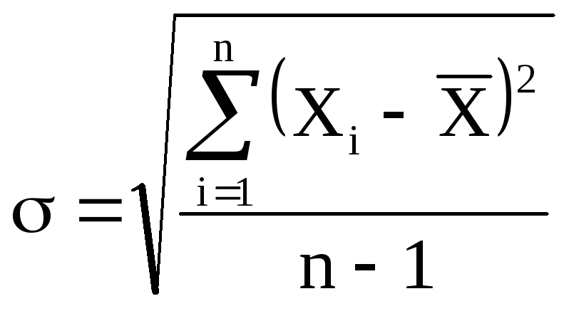
(5)
Величина
характеризует отклонение отдельного
единичного измерения от истинного
значения.
Если мы вычислили
по n
измерениям среднее значение
![]()
по формуле (2), то это значение будет
более точным, то есть будет меньше
отличаться от истинного, чем каждое
отдельное измерение. Средняя квадратичная
ошибка среднего значения
![]()
равна
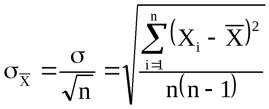
(6)
где — среднеквадратичная
ошибка каждого отдельного измерения,
n
– число
измерений.
Таким образом,
увеличивая число опытов, можно уменьшить
случайную ошибку в величине среднего
значения.
В настоящее время
результаты научных и технических
измерений принято представлять в виде
![]()
(7)
Как показывает
теория, при такой записи мы знаем
надежность полученного результата, а
именно, что истинная величина Х с
вероятностью 68% отличается от
![]()
не более, чем на
![]() .
.
При использовании
же средней арифметической (абсолютной)
ошибки (формула 2) о надежности результата
ничего сказать нельзя. Некоторое
представление о точности проведенных
измерений в этом случае дает относительная
ошибка (формула 4).
При выполнении
лабораторных работ студенты могут
использовать как среднюю абсолютную
ошибку, так и среднюю квадратичную.
Какую из них применять указывается
непосредственно в каждой конкретной
работе (или указывается преподавателем).
Обычно если число
измерений не превышает 3 – 5, то
можно использовать среднюю абсолютную
ошибку. Если число измерений порядка
10 и более, то следует использовать более
корректную оценку с
помощью средней квадратичной ошибки
среднего (формулы 5 и 6).
Учет систематических ошибок.
Увеличением числа
измерений можно уменьшить только
случайные ошибки опыта, но не
систематические.
Максимальное
значение систематической ошибки обычно
указывается на приборе или в его паспорте.
Для измерений с помощью обычной
металлической линейки систематическая
ошибка составляет не менее 0,5 мм; для
измерений штангенциркулем –
0,1 – 0,05 мм;
микрометром – 0,01 мм.
Часто в качестве
систематической ошибки берется половина
цены деления прибора.
На шкалах
электроизмерительных приборов указывается
класс точности. Зная класс точности К,
можно вычислить систематическую ошибку
прибора ∆Х по формуле
![]()
где К – класс
точности прибора, Хпр – предельное
значение величины, которое может быть
измерено по шкале прибора.
Так, амперметр
класса 0,5 со шкалой до 5А измеряет ток с
ошибкой не более
![]()
Среднее значение
полной погрешности складывается из
случайной и систематической
погрешностей.
![]()
Ответ с учетом
систематических и случайных ошибок
записывается в виде
![]()
Погрешности косвенных измерений
В физических
экспериментах чаще бывает так, что
искомая физическая величина сама на
опыте измерена быть не может, а является
функцией других величин, измеряемых
непосредственно. Например, чтобы
определить объём цилиндра, надо измерить
диаметр D и высоту h, а затем вычислить
объем по формуле
![]()
Величины D и h будут измерены с
некоторой ошибкой. Следовательно,
вычисленная величина
V
получится также с некоторой ошибкой.
Надо уметь выражать погрешность
вычисленной величины через погрешности
измеренных величин.
Как и при прямых
измерениях можно вычислять среднюю
абсолютную (среднюю арифметическую)
ошибку или среднюю квадратичную ошибку.
Общие правила
вычисления ошибок для обоих случаев
выводятся с помощью дифференциального
исчисления.
Пусть искомая
величина φ является функцией нескольких
переменных Х,
У, Z…
φ(Х,
У, Z…).
Путем прямых
измерений мы можем найти величины
![]() ,
,
а также оценить их средние абсолютные
ошибки
![]() …
…
или средние квадратичные ошибки Х,
У,
Z…
Тогда средняя
арифметическая погрешность
вычисляется по формуле
![]()
где
![]() — частные
— частные
производные от φ по
Х, У, Z. Они
вычисляются для средних значений
![]() …
…
Средняя квадратичная
погрешность вычисляется по формуле
![]()
Пример.
Выведем формулы погрешности для
вычисления объёма цилиндра.
а) Средняя
арифметическая погрешность.
Величины
D и h
измеряются соответственно с ошибкой
D
и h.
Погрешность
величины объёма будет равна
![]()
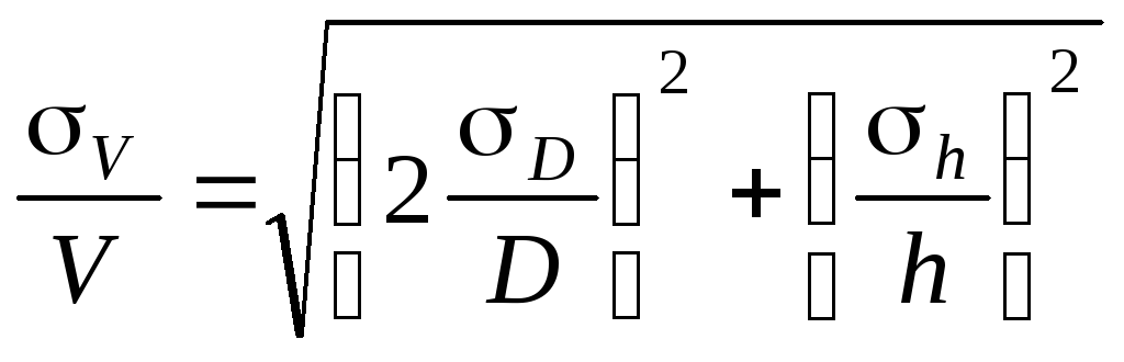
б) Средняя
квадратичная погрешность.
Величины
D и h
измеряются соответственно с ошибкой
D, h.
Погрешность
величины объёма будет равна
![]()
Если формула
представляет выражение удобное для
логарифмирования (то есть произведение,
дробь, степень), то удобнее вначале
вычислять относительную погрешность.
Для этого (в случае средней арифметической
погрешности) надо проделать следующее.
1. Прологарифмировать
выражение.
2. Продифференцировать
его.
3. Объединить
все члены с одинаковым дифференциалом
и вынести его за скобки.
4. Взять выражение
перед различными дифференциалами по
модулю.
5. Заменить
значки дифференциалов d
на значки абсолютной погрешности .
В итоге получится
формула для относительной погрешности
![]()
Затем,
зная ,
можно вычислить абсолютную погрешность
=
Пример.
![]()
![]()
![]()
![]()
Аналогично можно
записать относительную среднюю
квадратичную погрешность
Правила
представления результатов измерения
следующие:
-
погрешность должна
округляться до одной значащей цифры:
правильно = 0,04,
неправильно —
= 0,0382;
-
последняя значащая
цифра результата должна быть того же
порядка величины, что и погрешность:
правильно
= 9,830,03,
неправильно —
= 9,8260,03;
-
если результат
имеет очень большую или очень малую
величину, необходимо использовать
показательную форму записи — одну и ту
же для результата и его погрешности,
причем запятая десятичной дроби должна
следовать за первой значащей цифрой
результата:
правильно —
= (5,270,03)10-5,
неправильно —
= 0,00005270,0000003,
= 5,2710-50,0000003,
=
= 0,0000527310-7,
= (5273)10-7,
= (0,5270,003)
10-4.
-
Если результат
имеет размерность, ее необходимо
указать:
правильно – g=(9,820,02)
м/c2,
неправильно – g=(9,820,02).
Соседние файлы в папке Отчеты_Погрешность
- #
- #
- #
- #
- #
Среднеквадратичная ошибка (Mean Squared Error) – Среднее арифметическое (Mean) квадратов разностей между предсказанными и реальными значениями Модели (Model) Машинного обучения (ML):

Рассчитывается с помощью формулы, которая будет пояснена в примере ниже:
$$MSE = frac{1}{n} × sum_{i=1}^n (y_i — widetilde{y}_i)^2$$
$$MSEspace{}{–}space{Среднеквадратическая}space{ошибка,}$$
$$nspace{}{–}space{количество}space{наблюдений,}$$
$$y_ispace{}{–}space{фактическая}space{координата}space{наблюдения,}$$
$$widetilde{y}_ispace{}{–}space{предсказанная}space{координата}space{наблюдения,}$$
MSE практически никогда не равен нулю, и происходит это из-за элемента случайности в данных или неучитывания Оценочной функцией (Estimator) всех факторов, которые могли бы улучшить предсказательную способность.
Пример. Исследуем линейную регрессию, изображенную на графике выше, и установим величину среднеквадратической Ошибки (Error). Фактические координаты точек-Наблюдений (Observation) выглядят следующим образом:

Мы имеем дело с Линейной регрессией (Linear Regression), потому уравнение, предсказывающее положение записей, можно представить с помощью формулы:
$$y = M * x + b$$
$$yspace{–}space{значение}space{координаты}space{оси}space{y,}$$
$$Mspace{–}space{уклон}space{прямой}$$
$$xspace{–}space{значение}space{координаты}space{оси}space{x,}$$
$$bspace{–}space{смещение}space{прямой}space{относительно}space{начала}space{координат}$$
Параметры M и b уравнения нам, к счастью, известны в данном обучающем примере, и потому уравнение выглядит следующим образом:
$$y = 0,5252 * x + 17,306$$
Зная координаты реальных записей и уравнение линейной регрессии, мы можем восстановить полные координаты предсказанных наблюдений, обозначенных серыми точками на графике выше. Простой подстановкой значения координаты x в уравнение мы рассчитаем значение координаты ỹ:

Рассчитаем квадрат разницы между Y и Ỹ:

Сумма таких квадратов равна 4 445. Осталось только разделить это число на количество наблюдений (9):
$$MSE = frac{1}{9} × 4445 = 493$$
Само по себе число в такой ситуации становится показательным, когда Дата-сайентист (Data Scientist) предпринимает попытки улучшить предсказательную способность модели и сравнивает MSE каждой итерации, выбирая такое уравнение, что сгенерирует наименьшую погрешность в предсказаниях.
MSE и Scikit-learn
Среднеквадратическую ошибку можно вычислить с помощью SkLearn. Для начала импортируем функцию:
import sklearn
from sklearn.metrics import mean_squared_error
Инициализируем крошечные списки, содержащие реальные и предсказанные координаты y:
y_true = [5, 41, 70, 77, 134, 68, 138, 101, 131]
y_pred = [23, 35, 55, 90, 93, 103, 118, 121, 129]
Инициируем функцию mean_squared_error(), которая рассчитает MSE тем же способом, что и формула выше:
mean_squared_error(y_true, y_pred)
Интересно, что конечный результат на 3 отличается от расчетов с помощью Apple Numbers:
496.0Ноутбук, не требующий дополнительной настройки на момент написания статьи, можно скачать здесь.
Автор оригинальной статьи: @mmoshikoo
Фото: @tobyelliott
Средняя квадратичная ошибка.
При ответственных
измерениях, когда необходимо знать
надежность полученных результатов,
используется средняя квадратичная
ошибка (или
стандартное отклонение), которая
определяется формулой
(5)
Величина
характеризует отклонение отдельного
единичного измерения от истинного
значения.
Если мы вычислили
по n
измерениям среднее значение
![]()
по формуле (2), то это значение будет
более точным, то есть будет меньше
отличаться от истинного, чем каждое
отдельное измерение. Средняя квадратичная
ошибка среднего значения
![]()
равна
(6)
где — среднеквадратичная
ошибка каждого отдельного измерения,
n
– число
измерений.
Таким образом,
увеличивая число опытов, можно уменьшить
случайную ошибку в величине среднего
значения.
В настоящее время
результаты научных и технических
измерений принято представлять в виде
![]()
(7)
Как показывает
теория, при такой записи мы знаем
надежность полученного результата, а
именно, что истинная величина Х с
вероятностью 68% отличается от
![]()
не более, чем на
![]() .
.
При использовании
же средней арифметической (абсолютной)
ошибки (формула 2) о надежности результата
ничего сказать нельзя. Некоторое
представление о точности проведенных
измерений в этом случае дает относительная
ошибка (формула 4).
При выполнении
лабораторных работ студенты могут
использовать как среднюю абсолютную
ошибку, так и среднюю квадратичную.
Какую из них применять указывается
непосредственно в каждой конкретной
работе (или указывается преподавателем).
Обычно если число
измерений не превышает 3 – 5, то
можно использовать среднюю абсолютную
ошибку. Если число измерений порядка
10 и более, то следует использовать более
корректную оценку с
помощью средней квадратичной ошибки
среднего (формулы 5 и 6).
Учет систематических ошибок.
Увеличением числа
измерений можно уменьшить только
случайные ошибки опыта, но не
систематические.
Максимальное
значение систематической ошибки обычно
указывается на приборе или в его паспорте.
Для измерений с помощью обычной
металлической линейки систематическая
ошибка составляет не менее 0,5 мм; для
измерений штангенциркулем –
0,1 – 0,05 мм;
микрометром – 0,01 мм.
Часто в качестве
систематической ошибки берется половина
цены деления прибора.
На шкалах
электроизмерительных приборов указывается
класс точности. Зная класс точности К,
можно вычислить систематическую ошибку
прибора ∆Х по формуле
![]()
где К – класс
точности прибора, Хпр – предельное
значение величины, которое может быть
измерено по шкале прибора.
Так, амперметр
класса 0,5 со шкалой до 5А измеряет ток с
ошибкой не более
![]()
Среднее значение
полной погрешности складывается из
случайной и систематической
погрешностей.
![]()
Ответ с учетом
систематических и случайных ошибок
записывается в виде
![]()
Погрешности косвенных измерений
В физических
экспериментах чаще бывает так, что
искомая физическая величина сама на
опыте измерена быть не может, а является
функцией других величин, измеряемых
непосредственно. Например, чтобы
определить объём цилиндра, надо измерить
диаметр D и высоту h, а затем вычислить
объем по формуле
![]()
Величины D и h будут измерены с
некоторой ошибкой. Следовательно,
вычисленная величина
V
получится также с некоторой ошибкой.
Надо уметь выражать погрешность
вычисленной величины через погрешности
измеренных величин.
Как и при прямых
измерениях можно вычислять среднюю
абсолютную (среднюю арифметическую)
ошибку или среднюю квадратичную ошибку.
Общие правила
вычисления ошибок для обоих случаев
выводятся с помощью дифференциального
исчисления.
Пусть искомая
величина φ является функцией нескольких
переменных Х,
У, Z…
φ(Х,
У, Z…).
Путем прямых
измерений мы можем найти величины
![]() ,
,
а также оценить их средние абсолютные
ошибки
![]() …
…
или средние квадратичные ошибки Х,
У,
Z…
Тогда средняя
арифметическая погрешность
вычисляется по формуле
![]()
где
![]() — частные
— частные
производные от φ по
Х, У, Z. Они
вычисляются для средних значений
![]() …
…
Средняя квадратичная
погрешность вычисляется по формуле
![]()
Пример.
Выведем формулы погрешности для
вычисления объёма цилиндра.
а) Средняя
арифметическая погрешность.
Величины
D и h
измеряются соответственно с ошибкой
D
и h.
Погрешность
величины объёма будет равна
![]()
б) Средняя
квадратичная погрешность.
Величины
D и h
измеряются соответственно с ошибкой
D, h.
Погрешность
величины объёма будет равна
![]()
Если формула
представляет выражение удобное для
логарифмирования (то есть произведение,
дробь, степень), то удобнее вначале
вычислять относительную погрешность.
Для этого (в случае средней арифметической
погрешности) надо проделать следующее.
1. Прологарифмировать
выражение.
2. Продифференцировать
его.
3. Объединить
все члены с одинаковым дифференциалом
и вынести его за скобки.
4. Взять выражение
перед различными дифференциалами по
модулю.
5. Заменить
значки дифференциалов d
на значки абсолютной погрешности .
В итоге получится
формула для относительной погрешности
![]()
Затем,
зная ,
можно вычислить абсолютную погрешность
=
Пример.
![]()
![]()
![]()
![]()
Аналогично можно
записать относительную среднюю
квадратичную погрешность
Правила
представления результатов измерения
следующие:
-
погрешность должна
округляться до одной значащей цифры:
правильно = 0,04,
неправильно —
= 0,0382;
-
последняя значащая
цифра результата должна быть того же
порядка величины, что и погрешность:
правильно
= 9,830,03,
неправильно —
= 9,8260,03;
-
если результат
имеет очень большую или очень малую
величину, необходимо использовать
показательную форму записи — одну и ту
же для результата и его погрешности,
причем запятая десятичной дроби должна
следовать за первой значащей цифрой
результата:
правильно —
= (5,270,03)10-5,
неправильно —
= 0,00005270,0000003,
= 5,2710-50,0000003,
=
= 0,0000527310-7,
= (5273)10-7,
= (0,5270,003)
10-4.
-
Если результат
имеет размерность, ее необходимо
указать:
правильно – g=(9,820,02)
м/c2,
неправильно – g=(9,820,02).
Соседние файлы в папке Отчеты_Погрешность
- #
- #
- #
- #
- #
In statistics, the mean squared error (MSE)[1] or mean squared deviation (MSD) of an estimator (of a procedure for estimating an unobserved quantity) measures the average of the squares of the errors—that is, the average squared difference between the estimated values and the actual value. MSE is a risk function, corresponding to the expected value of the squared error loss.[2] The fact that MSE is almost always strictly positive (and not zero) is because of randomness or because the estimator does not account for information that could produce a more accurate estimate.[3] In machine learning, specifically empirical risk minimization, MSE may refer to the empirical risk (the average loss on an observed data set), as an estimate of the true MSE (the true risk: the average loss on the actual population distribution).
The MSE is a measure of the quality of an estimator. As it is derived from the square of Euclidean distance, it is always a positive value that decreases as the error approaches zero.
The MSE is the second moment (about the origin) of the error, and thus incorporates both the variance of the estimator (how widely spread the estimates are from one data sample to another) and its bias (how far off the average estimated value is from the true value).[citation needed] For an unbiased estimator, the MSE is the variance of the estimator. Like the variance, MSE has the same units of measurement as the square of the quantity being estimated. In an analogy to standard deviation, taking the square root of MSE yields the root-mean-square error or root-mean-square deviation (RMSE or RMSD), which has the same units as the quantity being estimated; for an unbiased estimator, the RMSE is the square root of the variance, known as the standard error.
Definition and basic properties[edit]
The MSE either assesses the quality of a predictor (i.e., a function mapping arbitrary inputs to a sample of values of some random variable), or of an estimator (i.e., a mathematical function mapping a sample of data to an estimate of a parameter of the population from which the data is sampled). The definition of an MSE differs according to whether one is describing a predictor or an estimator.
Predictor[edit]
If a vector of predictions is generated from a sample of data points on all variables, and is the vector of observed values of the variable being predicted, with being the predicted values (e.g. as from a least-squares fit), then the within-sample MSE of the predictor is computed as
In other words, the MSE is the mean of the squares of the errors . This is an easily computable quantity for a particular sample (and hence is sample-dependent).
In matrix notation,
where is and is the column vector.
The MSE can also be computed on q data points that were not used in estimating the model, either because they were held back for this purpose, or because these data have been newly obtained. Within this process, known as statistical learning, the MSE is often called the test MSE,[4] and is computed as
Estimator[edit]
The MSE of an estimator with respect to an unknown parameter is defined as[1]
This definition depends on the unknown parameter, but the MSE is a priori a property of an estimator. The MSE could be a function of unknown parameters, in which case any estimator of the MSE based on estimates of these parameters would be a function of the data (and thus a random variable). If the estimator is derived as a sample statistic and is used to estimate some population parameter, then the expectation is with respect to the sampling distribution of the sample statistic.
The MSE can be written as the sum of the variance of the estimator and the squared bias of the estimator, providing a useful way to calculate the MSE and implying that in the case of unbiased estimators, the MSE and variance are equivalent.[5]
Proof of variance and bias relationship[edit]
An even shorter proof can be achieved using the well-known formula that for a random variable , . By substituting with, , we have
But in real modeling case, MSE could be described as the addition of model variance, model bias, and irreducible uncertainty (see Bias–variance tradeoff). According to the relationship, the MSE of the estimators could be simply used for the efficiency comparison, which includes the information of estimator variance and bias. This is called MSE criterion.
In regression[edit]
In regression analysis, plotting is a more natural way to view the overall trend of the whole data. The mean of the distance from each point to the predicted regression model can be calculated, and shown as the mean squared error. The squaring is critical to reduce the complexity with negative signs. To minimize MSE, the model could be more accurate, which would mean the model is closer to actual data. One example of a linear regression using this method is the least squares method—which evaluates appropriateness of linear regression model to model bivariate dataset,[6] but whose limitation is related to known distribution of the data.
The term mean squared error is sometimes used to refer to the unbiased estimate of error variance: the residual sum of squares divided by the number of degrees of freedom. This definition for a known, computed quantity differs from the above definition for the computed MSE of a predictor, in that a different denominator is used. The denominator is the sample size reduced by the number of model parameters estimated from the same data, (n−p) for p regressors or (n−p−1) if an intercept is used (see errors and residuals in statistics for more details).[7] Although the MSE (as defined in this article) is not an unbiased estimator of the error variance, it is consistent, given the consistency of the predictor.
In regression analysis, «mean squared error», often referred to as mean squared prediction error or «out-of-sample mean squared error», can also refer to the mean value of the squared deviations of the predictions from the true values, over an out-of-sample test space, generated by a model estimated over a particular sample space. This also is a known, computed quantity, and it varies by sample and by out-of-sample test space.
Examples[edit]
Mean[edit]
Suppose we have a random sample of size from a population, . Suppose the sample units were chosen with replacement. That is, the units are selected one at a time, and previously selected units are still eligible for selection for all draws. The usual estimator for the is the sample average
which has an expected value equal to the true mean (so it is unbiased) and a mean squared error of
where is the population variance.
For a Gaussian distribution, this is the best unbiased estimator (i.e., one with the lowest MSE among all unbiased estimators), but not, say, for a uniform distribution.
Variance[edit]
The usual estimator for the variance is the corrected sample variance:
This is unbiased (its expected value is ), hence also called the unbiased sample variance, and its MSE is[8]
where is the fourth central moment of the distribution or population, and is the excess kurtosis.
However, one can use other estimators for which are proportional to , and an appropriate choice can always give a lower mean squared error. If we define
then we calculate:
This is minimized when
For a Gaussian distribution, where , this means that the MSE is minimized when dividing the sum by . The minimum excess kurtosis is ,[a] which is achieved by a Bernoulli distribution with p = 1/2 (a coin flip), and the MSE is minimized for Hence regardless of the kurtosis, we get a «better» estimate (in the sense of having a lower MSE) by scaling down the unbiased estimator a little bit; this is a simple example of a shrinkage estimator: one «shrinks» the estimator towards zero (scales down the unbiased estimator).
Further, while the corrected sample variance is the best unbiased estimator (minimum mean squared error among unbiased estimators) of variance for Gaussian distributions, if the distribution is not Gaussian, then even among unbiased estimators, the best unbiased estimator of the variance may not be
Gaussian distribution[edit]
The following table gives several estimators of the true parameters of the population, μ and σ2, for the Gaussian case.[9]
| True value | Estimator | Mean squared error |
|---|---|---|
|
= the unbiased estimator of the population mean, |
|
|
= the unbiased estimator of the population variance, |
|
|
= the biased estimator of the population variance, |
|
|
= the biased estimator of the population variance, |
|
Interpretation[edit]
An MSE of zero, meaning that the estimator predicts observations of the parameter with perfect accuracy, is ideal (but typically not possible).
Values of MSE may be used for comparative purposes. Two or more statistical models may be compared using their MSEs—as a measure of how well they explain a given set of observations: An unbiased estimator (estimated from a statistical model) with the smallest variance among all unbiased estimators is the best unbiased estimator or MVUE (Minimum-Variance Unbiased Estimator).
Both analysis of variance and linear regression techniques estimate the MSE as part of the analysis and use the estimated MSE to determine the statistical significance of the factors or predictors under study. The goal of experimental design is to construct experiments in such a way that when the observations are analyzed, the MSE is close to zero relative to the magnitude of at least one of the estimated treatment effects.
In one-way analysis of variance, MSE can be calculated by the division of the sum of squared errors and the degree of freedom. Also, the f-value is the ratio of the mean squared treatment and the MSE.
MSE is also used in several stepwise regression techniques as part of the determination as to how many predictors from a candidate set to include in a model for a given set of observations.
Applications[edit]
- Minimizing MSE is a key criterion in selecting estimators: see minimum mean-square error. Among unbiased estimators, minimizing the MSE is equivalent to minimizing the variance, and the estimator that does this is the minimum variance unbiased estimator. However, a biased estimator may have lower MSE; see estimator bias.
- In statistical modelling the MSE can represent the difference between the actual observations and the observation values predicted by the model. In this context, it is used to determine the extent to which the model fits the data as well as whether removing some explanatory variables is possible without significantly harming the model’s predictive ability.
- In forecasting and prediction, the Brier score is a measure of forecast skill based on MSE.
Loss function[edit]
Squared error loss is one of the most widely used loss functions in statistics[citation needed], though its widespread use stems more from mathematical convenience than considerations of actual loss in applications. Carl Friedrich Gauss, who introduced the use of mean squared error, was aware of its arbitrariness and was in agreement with objections to it on these grounds.[3] The mathematical benefits of mean squared error are particularly evident in its use at analyzing the performance of linear regression, as it allows one to partition the variation in a dataset into variation explained by the model and variation explained by randomness.
Criticism[edit]
The use of mean squared error without question has been criticized by the decision theorist James Berger. Mean squared error is the negative of the expected value of one specific utility function, the quadratic utility function, which may not be the appropriate utility function to use under a given set of circumstances. There are, however, some scenarios where mean squared error can serve as a good approximation to a loss function occurring naturally in an application.[10]
Like variance, mean squared error has the disadvantage of heavily weighting outliers.[11] This is a result of the squaring of each term, which effectively weights large errors more heavily than small ones. This property, undesirable in many applications, has led researchers to use alternatives such as the mean absolute error, or those based on the median.
See also[edit]
- Bias–variance tradeoff
- Hodges’ estimator
- James–Stein estimator
- Mean percentage error
- Mean square quantization error
- Mean square weighted deviation
- Mean squared displacement
- Mean squared prediction error
- Minimum mean square error
- Minimum mean squared error estimator
- Overfitting
- Peak signal-to-noise ratio
Notes[edit]
- ^ This can be proved by Jensen’s inequality as follows. The fourth central moment is an upper bound for the square of variance, so that the least value for their ratio is one, therefore, the least value for the excess kurtosis is −2, achieved, for instance, by a Bernoulli with p=1/2.
References[edit]
- ^ a b «Mean Squared Error (MSE)». www.probabilitycourse.com. Retrieved 2020-09-12.
- ^ Bickel, Peter J.; Doksum, Kjell A. (2015). Mathematical Statistics: Basic Ideas and Selected Topics. Vol. I (Second ed.). p. 20.
If we use quadratic loss, our risk function is called the mean squared error (MSE) …
- ^ a b Lehmann, E. L.; Casella, George (1998). Theory of Point Estimation (2nd ed.). New York: Springer. ISBN 978-0-387-98502-2. MR 1639875.
- ^ Gareth, James; Witten, Daniela; Hastie, Trevor; Tibshirani, Rob (2021). An Introduction to Statistical Learning: with Applications in R. Springer. ISBN 978-1071614174.
- ^ Wackerly, Dennis; Mendenhall, William; Scheaffer, Richard L. (2008). Mathematical Statistics with Applications (7 ed.). Belmont, CA, USA: Thomson Higher Education. ISBN 978-0-495-38508-0.
- ^ A modern introduction to probability and statistics : understanding why and how. Dekking, Michel, 1946-. London: Springer. 2005. ISBN 978-1-85233-896-1. OCLC 262680588.
{{cite book}}: CS1 maint: others (link) - ^ Steel, R.G.D, and Torrie, J. H., Principles and Procedures of Statistics with Special Reference to the Biological Sciences., McGraw Hill, 1960, page 288.
- ^ Mood, A.; Graybill, F.; Boes, D. (1974). Introduction to the Theory of Statistics (3rd ed.). McGraw-Hill. p. 229.
- ^ DeGroot, Morris H. (1980). Probability and Statistics (2nd ed.). Addison-Wesley.
- ^ Berger, James O. (1985). «2.4.2 Certain Standard Loss Functions». Statistical Decision Theory and Bayesian Analysis (2nd ed.). New York: Springer-Verlag. p. 60. ISBN 978-0-387-96098-2. MR 0804611.
- ^ Bermejo, Sergio; Cabestany, Joan (2001). «Oriented principal component analysis for large margin classifiers». Neural Networks. 14 (10): 1447–1461. doi:10.1016/S0893-6080(01)00106-X. PMID 11771723.
Среднеквадратичная ошибка (Mean Squared Error) – Среднее арифметическое (Mean) квадратов разностей между предсказанными и реальными значениями Модели (Model) Машинного обучения (ML):
Рассчитывается с помощью формулы, которая будет пояснена в примере ниже:
$$MSE = frac{1}{n} × sum_{i=1}^n (y_i — widetilde{y}_i)^2$$
$$MSEspace{}{–}space{Среднеквадратическая}space{ошибка,}$$
$$nspace{}{–}space{количество}space{наблюдений,}$$
$$y_ispace{}{–}space{фактическая}space{координата}space{наблюдения,}$$
$$widetilde{y}_ispace{}{–}space{предсказанная}space{координата}space{наблюдения,}$$
MSE практически никогда не равен нулю, и происходит это из-за элемента случайности в данных или неучитывания Оценочной функцией (Estimator) всех факторов, которые могли бы улучшить предсказательную способность.
Пример. Исследуем линейную регрессию, изображенную на графике выше, и установим величину среднеквадратической Ошибки (Error). Фактические координаты точек-Наблюдений (Observation) выглядят следующим образом:
Мы имеем дело с Линейной регрессией (Linear Regression), потому уравнение, предсказывающее положение записей, можно представить с помощью формулы:
$$y = M * x + b$$
$$yspace{–}space{значение}space{координаты}space{оси}space{y,}$$
$$Mspace{–}space{уклон}space{прямой}$$
$$xspace{–}space{значение}space{координаты}space{оси}space{x,}$$
$$bspace{–}space{смещение}space{прямой}space{относительно}space{начала}space{координат}$$
Параметры M и b уравнения нам, к счастью, известны в данном обучающем примере, и потому уравнение выглядит следующим образом:
$$y = 0,5252 * x + 17,306$$
Зная координаты реальных записей и уравнение линейной регрессии, мы можем восстановить полные координаты предсказанных наблюдений, обозначенных серыми точками на графике выше. Простой подстановкой значения координаты x в уравнение мы рассчитаем значение координаты ỹ:
Рассчитаем квадрат разницы между Y и Ỹ:
Сумма таких квадратов равна 4 445. Осталось только разделить это число на количество наблюдений (9):
$$MSE = frac{1}{9} × 4445 = 493$$
Само по себе число в такой ситуации становится показательным, когда Дата-сайентист (Data Scientist) предпринимает попытки улучшить предсказательную способность модели и сравнивает MSE каждой итерации, выбирая такое уравнение, что сгенерирует наименьшую погрешность в предсказаниях.
MSE и Scikit-learn
Среднеквадратическую ошибку можно вычислить с помощью SkLearn. Для начала импортируем функцию:
import sklearn
from sklearn.metrics import mean_squared_error
Инициализируем крошечные списки, содержащие реальные и предсказанные координаты y:
y_true = [5, 41, 70, 77, 134, 68, 138, 101, 131]
y_pred = [23, 35, 55, 90, 93, 103, 118, 121, 129]
Инициируем функцию mean_squared_error(), которая рассчитает MSE тем же способом, что и формула выше:
mean_squared_error(y_true, y_pred)
Интересно, что конечный результат на 3 отличается от расчетов с помощью Apple Numbers:
496.0Ноутбук, не требующий дополнительной настройки на момент написания статьи, можно скачать здесь.
Автор оригинальной статьи: @mmoshikoo
Фото: @tobyelliott
17 авг. 2022 г.
читать 3 мин
В статистике регрессионный анализ — это метод, который мы используем для понимания взаимосвязи между переменной-предиктором x и переменной отклика y.
Когда мы проводим регрессионный анализ, мы получаем модель, которая сообщает нам прогнозируемое значение для переменной ответа на основе значения переменной-предиктора.
Один из способов оценить, насколько «хорошо» наша модель соответствует заданному набору данных, — это вычислить среднеквадратичную ошибку , которая представляет собой показатель, который говорит нам, насколько в среднем наши прогнозируемые значения отличаются от наших наблюдаемых значений.
Формула для нахождения среднеквадратичной ошибки, чаще называемая RMSE , выглядит следующим образом:
СКО = √[ Σ(P i – O i ) 2 / n ]
куда:
- Σ — причудливый символ, означающий «сумма».
- P i — прогнозируемое значение для i -го наблюдения в наборе данных.
- O i — наблюдаемое значение для i -го наблюдения в наборе данных.
- n — размер выборки
Технические примечания:
- Среднеквадратичную ошибку можно рассчитать для любого типа модели, которая дает прогнозные значения, которые затем можно сравнить с наблюдаемыми значениями набора данных.
- Среднеквадратичную ошибку также иногда называют среднеквадратичным отклонением, которое часто обозначается аббревиатурой RMSD.
Далее рассмотрим пример расчета среднеквадратичной ошибки в Excel.
Как рассчитать среднеквадратичную ошибку в Excel
В Excel нет встроенной функции для расчета RMSE, но мы можем довольно легко вычислить его с помощью одной формулы. Мы покажем, как рассчитать RMSE для двух разных сценариев.
Сценарий 1
В одном сценарии у вас может быть один столбец, содержащий предсказанные значения вашей модели, и другой столбец, содержащий наблюдаемые значения. На изображении ниже показан пример такого сценария:
Если это так, то вы можете рассчитать RMSE, введя следующую формулу в любую ячейку, а затем нажав CTRL+SHIFT+ENTER:
=КОРЕНЬ(СУММСК(A2:A21-B2:B21) / СЧЕТЧ(A2:A21))
Это говорит нам о том, что среднеквадратическая ошибка равна 2,6646 .
Формула может показаться немного сложной, но она имеет смысл, если ее разобрать:
= КОРЕНЬ( СУММСК(A2:A21-B2:B21) / СЧЕТЧ(A2:A21) )
- Во-первых, мы вычисляем сумму квадратов разностей между прогнозируемыми и наблюдаемыми значениями, используя функцию СУММСК() .
- Затем мы делим на размер выборки набора данных, используя COUNTA() , который подсчитывает количество непустых ячеек в диапазоне.
- Наконец, мы извлекаем квадратный корень из всего вычисления, используя функцию SQRT() .
Сценарий 2
В другом сценарии вы, возможно, уже вычислили разницу между прогнозируемыми и наблюдаемыми значениями. В этом случае у вас будет только один столбец, отображающий различия.
На изображении ниже показан пример этого сценария. Прогнозируемые значения отображаются в столбце A, наблюдаемые значения — в столбце B, а разница между прогнозируемыми и наблюдаемыми значениями — в столбце D:
Если это так, то вы можете рассчитать RMSE, введя следующую формулу в любую ячейку, а затем нажав CTRL+SHIFT+ENTER:
=КОРЕНЬ(СУММСК(D2:D21) / СЧЕТЧ(D2:D21))
Это говорит нам о том, что среднеквадратическая ошибка равна 2,6646 , что соответствует результату, полученному в первом сценарии. Это подтверждает, что эти два подхода к расчету RMSE эквивалентны.
Формула, которую мы использовали в этом сценарии, лишь немного отличается от той, что мы использовали в предыдущем сценарии:
= КОРЕНЬ (СУММСК(D2 :D21) / СЧЕТЧ(D2:D21) )
- Поскольку мы уже рассчитали разницу между предсказанными и наблюдаемыми значениями в столбце D, мы можем вычислить сумму квадратов разностей с помощью функции СУММСК().только со значениями в столбце D.
- Затем мы делим на размер выборки набора данных, используя COUNTA() , который подсчитывает количество непустых ячеек в диапазоне.
- Наконец, мы извлекаем квадратный корень из всего вычисления, используя функцию SQRT() .
Как интерпретировать среднеквадратичную ошибку
Как упоминалось ранее, RMSE — это полезный способ увидеть, насколько хорошо регрессионная модель (или любая модель, которая выдает прогнозируемые значения) способна «соответствовать» набору данных.
Чем больше RMSE, тем больше разница между прогнозируемыми и наблюдаемыми значениями, а это означает, что модель регрессии хуже соответствует данным. И наоборот, чем меньше RMSE, тем лучше модель соответствует данным.
Может быть особенно полезно сравнить RMSE двух разных моделей друг с другом, чтобы увидеть, какая модель лучше соответствует данным.
Для получения дополнительных руководств по Excel обязательно ознакомьтесь с нашей страницей руководств по Excel , на которой перечислены все учебные пособия Excel по статистике.
![]()
Загрузить PDF
![]()
Загрузить PDF
После сбора данных их нужно проанализировать. Обычно нужно найти среднее значение, квадратичное отклонение и погрешность. Мы расскажем вам, как это сделать.
-

1
Запишите числовые значения, которые вы собираетесь анализировать. Мы проанализируем случайно подобранные числовые значения в качестве примера.
- Например, 5 школьникам был предложен письменный тест. Их результаты (в баллах по 100 бальной системе): 12, 55, 74, 79 и 90 баллов.
Реклама

-
1
Для того чтобы посчитать среднее значение, нужно сложить все имеющиеся числовые значения и разделить получившееся число на их количество.
- Среднее значение (μ) = Σ/N, где Σ сумма всех числовых значений, а N количество значений.
- То есть, в нашем случае μ равно (12+55+74+79+90)/5 = 62.

-
1
Мы будем считать среднее отклонение. Среднее отклонение = σ = квадратный корень из [(Σ((X-μ)^2))/(N)].
- Для вышеуказанного примера это квадратный корень из [((12-62)^2 + (55-62)^2 + (74-62)^2 + (79-62)^2 + (90-62)^2)/(5)] = 27,4. (Обратите внимание, что если это выборочное среднеквадратическое отклонение, то делить нужно на N-1, где N количество значений.)
Реклама

-
1
Считаем среднюю погрешность (среднего значения). Это оценка того, насколько сильно округляется общее среднее значение. Чем больше числовых значений, тем меньше средняя погрешность, тем точнее среднее значение. Для расчета погрешности надо разделить среднее отклонение на корень квадратный от N. Стандартная погрешность = σ/кв.корень(n).
- Если в нашем примере 5 школьников, а всего в классе 50 школьников, и среднее отклонение, посчитанное для 50 школьников равно 17 (σ = 21), средняя погрешность = 17/кв. корень(5) = 7.6.

Советы
- Расчеты среднего значения, среднего отклонения и погрешности годятся для анализа равномерно распределенных данных. Среднее отклонение математического среднего значения распределения относится приблизительно к 68% данных, 2 средних отклонения – к 95% данных, а 3 – к 99.7% данных. Стандартная погрешность же уменьшается при увеличении количества значений.
- Простой в использовании калькулятор для расчета среднего отклонения.
Реклама
Предупреждения
- Считайте дважды. Все делают ошибки.
Реклама
Об этой статье
Эту страницу просматривали 65 201 раз.
Была ли эта статья полезной?
В статистика, то среднеквадратичная ошибка (MSE)[1][2] или среднеквадратическое отклонение (MSD) из оценщик (процедуры оценки ненаблюдаемой величины) измеряет средний квадратов ошибки — то есть средний квадрат разницы между оценочными и фактическими значениями. MSE — это функция риска, соответствующий ожидаемое значение квадрата ошибки потери. Тот факт, что MSE почти всегда строго положительный (а не нулевой), объясняется тем, что случайность или потому что оценщик не учитывает информацию это может дать более точную оценку.[3]
MSE — это мера качества оценки — она всегда неотрицательна, а значения, близкие к нулю, лучше.
МСЭ — второй момент (о происхождении) ошибки и, таким образом, включает в себя как отклонение оценщика (насколько разбросаны оценки от одного образец данных другому) и его предвзятость (насколько далеко среднее оценочное значение от истинного значения). Для объективный оценщик, MSE — это дисперсия оценки. Как и дисперсия, MSE имеет те же единицы измерения, что и квадрат оцениваемой величины. По аналогии с стандартное отклонение, извлечение квадратного корня из MSE дает среднеквадратичную ошибку или среднеквадратичное отклонение (RMSE или RMSD), который имеет те же единицы, что и оцениваемое количество; для несмещенной оценки RMSE — это квадратный корень из отклонение, известный как стандартная ошибка.
Определение и основные свойства
MSE либо оценивает качество предсказатель (т.е. функция, отображающая произвольные входные данные в выборку значений некоторых случайная переменная ) или оценщик (т.е. математическая функция отображение образец данных для оценки параметр из численность населения из которого берутся данные). Определение MSE различается в зависимости от того, описывается ли предсказатель или оценщик.
Предсказатель
Если вектор прогнозы генерируются из выборки п точки данных по всем переменным, и — вектор наблюдаемых значений прогнозируемой переменной, при этом будучи предсказанными значениями (например, по методу наименьших квадратов), то MSE в пределах выборки предсказателя вычисляется как

Другими словами, MSE — это иметь в виду  из квадраты ошибок
  . Это легко вычисляемая величина для конкретного образца (и, следовательно, зависит от образца).
В матрица обозначение
куда является и это матрица.
MSE также можно вычислить на q точки данных, которые не использовались при оценке модели, либо потому, что они были задержаны для этой цели, либо потому, что эти данные были получены заново. В этом процессе (известном как перекрестная проверка ), MSE часто называют среднеквадратичная ошибка прогноза, и вычисляется как

Оценщик
MSE оценщика по неизвестному параметру определяется как[2]
Это определение зависит от неизвестного параметра, но MSE априори свойство оценщика. MSE может быть функцией неизвестных параметров, и в этом случае любой оценщик MSE на основе оценок этих параметров будет функцией данных (и, следовательно, случайной величиной). Если оценщик выводится как статистика выборки и используется для оценки некоторого параметра совокупности, тогда ожидание относится к распределению выборки статистики выборки.
MSE можно записать как сумму отклонение оценщика и квадрата предвзятость оценщика, обеспечивая полезный способ вычисления MSE и подразумевая, что в случае несмещенных оценок MSE и дисперсия эквивалентны.[4]
Доказательство отношения дисперсии и предвзятости
- В качестве альтернативы у нас есть

Но в реальном случае моделирования MSE можно описать как добавление дисперсии модели, систематической ошибки модели и неснижаемой неопределенности. Согласно соотношению, MSE оценщиков может быть просто использована для эффективность сравнение, которое включает информацию о дисперсии и смещении оценки. Это называется критерием MSE.
В регрессе
В регрессивный анализ, построение графиков — более естественный способ просмотра общей тенденции всех данных. Среднее значение расстояния от каждой точки до прогнозируемой регрессионной модели может быть вычислено и показано как среднеквадратичная ошибка. Возведение в квадрат критически важно для уменьшения сложности с отрицательными знаками. Чтобы свести к минимуму MSE, модель может быть более точной, что означает, что модель ближе к фактическим данным. Одним из примеров линейной регрессии с использованием этого метода является метод наименьших квадратов —Который оценивает соответствие модели линейной регрессии модели двумерный набор данных[5], но чье ограничение связано с известным распределением данных.
Период, термин среднеквадратичная ошибка иногда используется для обозначения объективной оценки дисперсии ошибки: остаточная сумма квадратов делится на количество степени свободы. Это определение известной вычисленной величины отличается от приведенного выше определения вычисленной MSE предиктора тем, что используется другой знаменатель. Знаменатель — это размер выборки, уменьшенный на количество параметров модели, оцененных на основе тех же данных, (н-р) за п регрессоры или (п-п-1) если используется перехват (см. ошибки и остатки в статистике Больше подробностей).[6] Хотя MSE (как определено в этой статье) не является объективной оценкой дисперсии ошибки, она последовательный, учитывая непротиворечивость предсказателя.
В регрессионном анализе «среднеквадратичная ошибка», часто называемая среднеквадратичная ошибка прогноза или «среднеквадратичная ошибка вне выборки», также может относиться к среднему значению квадратичные отклонения прогнозов на основе истинных значений в тестовом пространстве вне выборки, сгенерированных моделью, оцененной в конкретном пространстве выборки. Это также известная вычисляемая величина, которая зависит от образца и тестового пространства вне образца.
Примеры
Иметь в виду
Предположим, у нас есть случайная выборка размера от населения, . Предположим, что образцы были выбраны с заменой. Это единицы выбираются по одному, и ранее выбранные единицы по-прежнему имеют право на выбор для всех рисует. Обычная оценка для это среднее по выборке[1]
ожидаемое значение которого равно истинному среднему значению (так что это беспристрастно) и среднеквадратичная ошибка
куда это дисперсия населения.
Для Гауссово распределение, это лучший объективный оценщик (то есть с самой низкой MSE среди всех несмещенных оценок), но не, скажем, для равномерное распределение.
Дисперсия
Обычной оценкой дисперсии является исправлено выборочная дисперсия:
Это объективно (его ожидаемое значение ), поэтому также называется объективная дисперсия выборки, и его MSE[7]
куда это четвертый центральный момент распределения или населения, и это избыточный эксцесс.
Однако можно использовать другие оценки для которые пропорциональны , и соответствующий выбор всегда может дать более низкую среднеквадратичную ошибку. Если мы определим
затем рассчитываем:
Это сводится к минимуму, когда
Для Гауссово распределение, куда , это означает, что MSE минимизируется при делении суммы на . Минимальный избыточный эксцесс составляет ,[а] что достигается за счет Распределение Бернулли с п = 1/2 (подбрасывание монеты), и MSE минимизируется для Следовательно, независимо от эксцесса, мы получаем «лучшую» оценку (в смысле наличия более низкой MSE), немного уменьшая несмещенную оценку; это простой пример оценщик усадки: один «сжимает» оценку до нуля (уменьшает несмещенную оценку).
Далее, хотя исправленная дисперсия выборки является лучший объективный оценщик (минимальная среднеквадратичная ошибка среди несмещенных оценок) дисперсии для гауссовских распределений, если распределение не является гауссовым, то даже среди несмещенных оценок лучшая несмещенная оценка дисперсии может не быть
Гауссово распределение
В следующей таблице приведены несколько оценок истинных параметров популяции, μ и σ.2, для гауссова случая.[8]
| Истинное значение | Оценщик | Среднеквадратичная ошибка |
|---|---|---|
|
= несмещенная оценка Средняя численность населения, |
|
|
= несмещенная оценка дисперсия населения, |
|
|
= смещенная оценка дисперсия населения, |
|
|
= смещенная оценка дисперсия населения, |
|
Интерпретация
MSE равна нулю, что означает, что оценщик предсказывает наблюдения параметра с идеальной точностью идеален (но обычно невозможен).
Значения MSE могут использоваться для сравнительных целей. Два и более статистические модели можно сравнить, используя их MSE — как меру того, насколько хорошо они объясняют данный набор наблюдений: несмещенная оценка (рассчитанная на основе статистической модели) с наименьшей дисперсией среди всех несмещенных оценок — это оценка лучший объективный оценщик или MVUE (несмещенная оценка минимальной дисперсии).
Обе линейная регрессия методы, такие как дисперсионный анализ оценить MSE как часть анализа и использовать оценочную MSE для определения Статистическая значимость изучаемых факторов или предикторов. Цель экспериментальная конструкция состоит в том, чтобы построить эксперименты таким образом, чтобы при анализе наблюдений MSE была близка к нулю относительно величины по крайней мере одного из оцененных эффектов лечения.
В односторонний дисперсионный анализ, MSE можно вычислить путем деления суммы квадратов ошибок и степени свободы. Кроме того, значение f — это отношение среднего квадрата обработки и MSE.
MSE также используется в нескольких пошаговая регрессия методы как часть определения того, сколько предикторов из набора кандидатов включить в модель для данного набора наблюдений.
Приложения
- Минимизация MSE является ключевым критерием при выборе оценщиков: см. минимальная среднеквадратичная ошибка. Среди несмещенных оценщиков минимизация MSE эквивалентна минимизации дисперсии, а оценщик, который делает это, является несмещенная оценка минимальной дисперсии. Однако смещенная оценка может иметь более низкую MSE; видеть систематическая ошибка оценки.
- В статистическое моделирование MSE может представлять разницу между фактическими наблюдениями и значениями наблюдений, предсказанными моделью. В этом контексте он используется для определения степени, в которой модель соответствует данным, а также возможности удаления некоторых объясняющих переменных без значительного ущерба для прогнозирующей способности модели.
- В прогнозирование и прогноз, то Оценка Бриера это мера умение прогнозировать на основе MSE.
Функция потерь
Квадратичная потеря ошибок — одна из наиболее широко используемых функции потерь в статистике[нужна цитата ], хотя его широкое использование проистекает больше из математического удобства, чем из соображений реальных потерь в приложениях. Карл Фридрих Гаусс, который ввел использование среднеквадратичной ошибки, сознавал ее произвол и был согласен с возражениями против нее на этих основаниях.[3] Математические преимущества среднеквадратичной ошибки особенно очевидны при ее использовании при анализе производительности линейная регрессия, поскольку он позволяет разделить вариацию в наборе данных на вариации, объясняемые моделью, и вариации, объясняемые случайностью.
Критика
Использование среднеквадратичной ошибки без вопросов подвергалось критике со стороны теоретик решений Джеймс Бергер. Среднеквадратичная ошибка — это отрицательное значение ожидаемого значения одного конкретного вспомогательная функция, квадратичная функция полезности, которая может не подходить для использования в данном наборе обстоятельств. Однако есть некоторые сценарии, в которых среднеквадратичная ошибка может служить хорошим приближением к функции потерь, естественным образом возникающей в приложении.[9]
подобно отклонение, среднеквадратичная ошибка имеет тот недостаток, что выбросы.[10] Это результат возведения в квадрат каждого члена, который фактически дает больший вес большим ошибкам, чем малым. Это свойство, нежелательное для многих приложений, заставило исследователей использовать альтернативы, такие как средняя абсолютная ошибка, или основанные на медиана.
Смотрите также
- Компромисс смещения и дисперсии
- Оценщик Ходжеса
- Оценка Джеймса – Стейна
- Средняя процентная ошибка
- Среднеквадратичная ошибка квантования
- Среднеквадратичное взвешенное отклонение
- Среднеквадратичное смещение
- Среднеквадратичная ошибка прогноза
- Минимальная среднеквадратичная ошибка
- Оценщик минимальной среднеквадратичной ошибки
- Пиковое отношение сигнал / шум
Примечания
- ^ Это может быть доказано Неравенство Дженсена следующим образом. Четвертый центральный момент является верхней границей квадрата дисперсии, так что наименьшее значение для их отношения равно единице, следовательно, наименьшее значение для избыточный эксцесс равно −2, что достигается, например, Бернулли с п=1/2.
Рекомендации
- ^ а б «Список вероятностных и статистических символов». Математическое хранилище. 2020-04-26. Получено 2020-09-12.
- ^ а б «Среднеквадратичная ошибка (MSE)». www.probabilitycourse.com. Получено 2020-09-12.
- ^ а б Lehmann, E. L .; Казелла, Джордж (1998). Теория точечного оценивания (2-е изд.). Нью-Йорк: Спрингер. ISBN 978-0-387-98502-2. Г-Н 1639875.
- ^ Вакерли, Деннис; Менденхолл, Уильям; Шеаффер, Ричард Л. (2008). Математическая статистика с приложениями (7-е изд.). Белмонт, Калифорния, США: Высшее образование Томсона. ISBN 978-0-495-38508-0.
- ^ Современное введение в вероятность и статистику: понимание, почему и как. Деккинг, Мишель, 1946-. Лондон: Спрингер. 2005 г. ISBN 978-1-85233-896-1. OCLC 262680588.CS1 maint: другие (ссылка на сайт)
- ^ Стил, Р.Г.Д., и Торри, Дж. Х., Принципы и процедуры статистики с особым акцентом на биологические науки., Макгроу Хилл, 1960, стр.288.
- ^ Настроение, А .; Graybill, F .; Боэс, Д. (1974). Введение в теорию статистики (3-е изд.). Макгроу-Хилл. п.229.
- ^ ДеГрут, Моррис Х. (1980). вероятность и статистика (2-е изд.). Эддисон-Уэсли.
- ^ Бергер, Джеймс О. (1985). «2.4.2 Некоторые стандартные функции потерь». Статистическая теория принятия решений и байесовский анализ (2-е изд.). Нью-Йорк: Springer-Verlag. п.60. ISBN 978-0-387-96098-2. Г-Н 0804611.
- ^ Бермехо, Серхио; Кабестани, Джоан (2001). «Ориентированный анализ главных компонентов для классификаторов с большой маржой». Нейронные сети. 14 (10): 1447–1461. Дои:10.1016 / S0893-6080 (01) 00106-X. PMID 11771723.