Excel для Microsoft 365 Excel для Microsoft 365 для Mac Excel для Интернета Excel для iPad Excel Web App Excel для iPhone Excel для планшетов с Android Excel для телефонов с Android Еще…Меньше
Формула с пролитой массивом, в который вы попытались ввести формулу, выходит за пределы диапазона. Попробуйте еще раз с небольшим диапазоном или массивом.
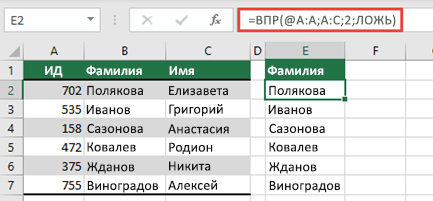
В следующем примере при перемещении формулы в ячейку F1 ошибка будет исправлена, и формула будет переносима правильно.
Распространенные причины: полные ссылки на столбцы
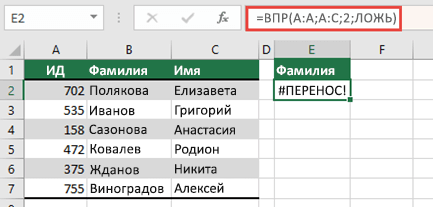
При создании формул в lookup_value в них часто неправильно засоряются. Перед динамическим массивом Приложение Excel учитывало только значение в той же строке, что и формулу, и игнорировало все остальные, так как при функции ВЛОП ожидалось только одно значение. При вводе динамических массивов Excel рассматривает все значения, предоставляемые lookup_value. Это означает, что если в качестве аргумента lookup_value столбец, Excel попытается найти все 1 048 576 значений в столбце. Когда все будет готово, он попытается пролить их на сетку и, скорее всего, зажмет #SPILL! ошибка «#ЗНАЧ!».
Например, при размещении в ячейке E2, как по примеру ниже, формула =ВЛОЖЕННАЯ(A:A;A:C;2;ЛОЖЬ) ранее только подыскала бы ИД в ячейке A2. Однако в динамическом массиве Excel формула приведет к #SPILL! из-за того, что Excel подытнет весь столбец, отвернет результат с результатом 1 048 576 и пожмет в конце сетки Excel.
Существует три простых способа решения этой проблемы:
|
# |
Подход |
Формула |
|---|---|---|
|
1 |
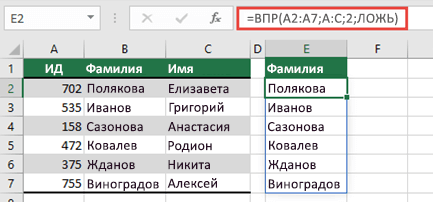
Ссылаясь только на значения подпапок, которые вас интересуют. Этот стиль формулы возвращает динамический массив, ноне работает с таблицами Excel.
|
=В ПРОСМОТР(A2:A7;A:C;2;ЛОЖЬ) |
|
2 |
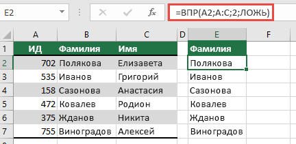
Ссылаясь только на значение в той же строке, скопируйте формулу вниз. Этот традиционный стиль формул работает в таблицах,но не возвращаетдинамический массив.
|
=В ПРОСМОТР(A2;A:C;2;ЛОЖЬ) |
|
3 |
Запрос на выполнение неявного пересечения с помощью оператора @ и копирование формулы вниз. Этот стиль формулы работает в таблицах,но не возвращаетдинамический массив.
|
=ВЛ.В.@A:A;A:C;2;ЛОЖЬ) |
Дополнительные сведения
Вы всегда можете задать вопрос специалисту Excel Tech Community, попросить помощи в сообществе Answers community, а также предложить новую функцию или улучшение на веб-сайте Excel User Voice.
См. также
Функция ФИЛЬТР
Функция СЛУЧМАССИВ
Функция ПОСЛЕДОВ
Функция СОРТ
Функция СОРТПО
Функция УНИК
Ошибки #ПЕРЕНОС! в Excel
Динамические массивы и поведение рассеянного массива
Неявное пересечение: @
Нужна дополнительная помощь?
Нужны дополнительные параметры?
Изучите преимущества подписки, просмотрите учебные курсы, узнайте, как защитить свое устройство и т. д.
В сообществах можно задавать вопросы и отвечать на них, отправлять отзывы и консультироваться с экспертами разных профилей.

Резюме
Ошибка #SPILL возникает, когда диапазон разлива блокируется чем-то на листе. Решение обычно состоит в том, чтобы очистить зону разлива от любых препятствующих данных. См. Ниже дополнительную информацию и инструкции по устранению.
Объяснение
О разливе и # РАЗЛИВ! ошибка
С появлением в Excel динамических массивов формулы, возвращающие несколько значений, «переносят» эти значения непосредственно на рабочий лист. Прямоугольник, в котором заключены значения, называется «диапазоном разлива». При изменении данных диапазон разлива будет расширяться или сокращаться по мере необходимости. Вы можете увидеть добавленные новые значения или исчезновение существующих.
Видео: Разлив и дальность разлива
Ошибка #SPILL возникает, когда диапазон разлива блокируется чем-то на листе. Иногда этого ожидают. Например, вы ввели формулу, ожидая, что она разразится, но существующие данные на листе мешают. Решение состоит в том, чтобы просто очистить зону разлива от любых мешающих данных.
Однако иногда ошибка может быть неожиданной и поэтому сбивать с толку. Прочтите ниже, как может быть вызвана эта ошибка и что вы можете сделать для ее устранения.
Поведение при разливе является естественным
Важно понимать, что поведение разлива является автоматическим и естественным. В динамическом Excel (в настоящее время только в Office 365 Excel) любая формула, даже простая формула без функций, может сказаться на результатах. Несмотря на то, что есть способы запретить формуле возвращать несколько результатов, отключение самого разлива с помощью глобального параметра невозможно.
Точно так же в Excel нет возможности «отключить ошибки #SPILL». Чтобы исправить ошибку #SPILL, вам необходимо изучить и устранить основную причину проблемы.
Исправление №1 — очистить зону разлива
Это самый простой для решения случай. Формула должна содержать несколько значений, но вместо этого возвращает #SPILL! потому что что-то мешает. Чтобы устранить ошибку, выберите любую ячейку в диапазоне разлива, чтобы видеть ее границы. Затем либо переместите данные блокировки в новое место, либо удалите данные полностью. Обратите внимание, что ячейки в диапазоне разлива должны быть пустыми, поэтому обратите внимание на ячейки, содержащие невидимые символы, например пробелы.
На приведенном ниже экране «x» блокирует диапазон разлива:

После удаления символа «x» функция UNIQUE обычно выдаёт результаты:

Исправление # 2 — добавить символ @
До появления динамических массивов Excel молча применял поведение, называемое «неявным пересечением», чтобы гарантировать, что определенные формулы, которые могут возвращать несколько результатов, возвращают только один результат. В Excel с нединамическими массивами эти формулы возвращают нормальный результат без ошибок. Однако в некоторых случаях та же формула, введенная в Dynamic Excel, может вызвать ошибку #SPILL. Например, на экране ниже ячейка D5 содержит скопированную формулу:
=$B$5:$B$10+3

Эта формула не вызовет ошибки, скажем, в Excel 2016, поскольку неявное пересечение не позволит формуле возвращать несколько результатов. Однако в Dynamic Excel формула автоматически возвращает несколько результатов на рабочий лист, которые врезаются друг в друга, поскольку формула копируется из D5: D10.
Одно из решений — использовать символ @, чтобы включить неявное пересечение, например:
= @$B$5:$B$10+3
С этим изменением каждая формула снова возвращает один результат, и ошибка #SPILL исчезает.

Примечание. Это частично объясняет, почему вы можете внезапно увидеть символ «@» в формулах, созданных в более ранних версиях Excel. Это сделано для сохранения совместимости. Поскольку формулы в более ранних версиях Excel не могут быть разделены на несколько ячеек, добавляется символ @, чтобы обеспечить такое же поведение при открытии формулы в динамическом Excel.
Исправление # 3 — формула встроенного динамического массива
Другой (лучший) способ исправить ошибку #SPILL, показанную выше, — использовать формулу встроенного динамического массива в D5 следующим образом:
=B5:B10+3
В динамическом Excel эта единственная формула передаст результаты в диапазон D5: D10, как показано на снимке экрана ниже:

Обратите внимание, что нет необходимости использовать абсолютную ссылку.
Explanation
About spilling and the #SPILL! error
With the introduction of Dynamic Arrays in Excel, formulas that return multiple values «spill» these values directly onto the worksheet. The rectangle that encloses the values is called the «spill range». When data changes, the spill range will expand or contract as needed. You might see new values added, or existing values disappear.
Video: Spilling and the spill range
Spill behavior is native
It’s important to understand that spill behavior is automatic and native. In Dynamic Excel (Excel 365/2021) any formula, even a simple formula without functions, can spill results. Although there are ways to stop a formula from returning multiple results, spilling itself can’t be disabled with a global setting. Similarly, there is no option in Excel to «disable #SPILL errors. To fix a #SPILL error, you’ll have to investigate and resolve the root cause of the problem.
Spill error information
A #SPILL error often occurs when a spill range is blocked by something on the worksheet. Sometimes this is expected. For example, you have entered a formula, expecting it to spill, but existing data in the worksheet is in the way. The solution is just to clear the spill range of any obstructing data. Less often, a #SPILL error has another cause. You can click the spill error indicator to see more information about the cause of the error:

Read below for more information about #SPILL! errors and the specific fixes.
1. Spill range blocked
This is the simplest case to resolve. The formula should return multiple values, but instead it returns #SPILL! because there is already something in the spill range. In the screen below, the «x» is blocking the spill range:

To fix the error, select any cell in the spill range so you can see its boundaries. Then make sure all cells in the spill range are empty. Once the «x» is removed, the UNIQUE function spills results normally:

Cells in the spill range must be empty, so be alert to cells with invisible characters, like spaces.
2. Excel Tables do not support dynamic arrays
Dynamic array formulas are not compatible with Excel tables. If you try to add a dynamic array formula to an Excel Table, the formula will return a #SPILL! error in all rows. The solution in this case is to (1) use an alternative formula or (2) remove the Excel Table by converting it to a normal range with the Convert to Range button on the Table Design tab of the Ribbon: Table Design > Convert to Range
Video: How to remove an Excel Table.
3. Spill range is unknown
Some functions are volatile and can’t be used with dynamic array functions because the result would be «unknown» and dynamic formulas do not currently support arrays of unknown length. For example, the following formula will return a #SPILL! error:
=SEQUENCE(RANDBETWEEN(1,100))
This happens because RANDBETWEEN is volatile and the array returned by SEQUENCE would therefore have an unknown length. The only solution is to avoid dynamic array formulas that create arrays or ranges of an unknown length.
4. Spill range too big
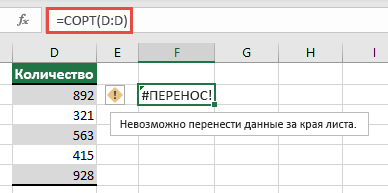
It is possible to write a formula that creates a spill range that extends off the edge of the worksheet. For example, the following formula uses the full column reference A:A:
=A:A+1
If this formula is entered in any row except row 1, it will return a #SPILL! error with a «Spill range is too big» message. This happens because the resulting spill range includes 1,048,576 rows (the limit in Excel) and will run off the bottom of the worksheet. Similarly, the formula below tries to use SEQUENCE to create an array with 17,000 columns:
=SEQUENCE(1,17000)
Because an Excel worksheet contains only 16,384 columns, this formula also returns a #SPILL! error. The solution is to avoid references and formulas that may create spill ranges that do not fit on the worksheet.
5. Implicit intersection (@)
Before Dynamic Arrays, Excel silently applied a behavior called «implicit intersection» to ensure that certain formulas with the potential to return multiple results only returned a single result. In non-dynamic array Excel, these formulas return a normal-looking result with no error. However, in certain cases the same formula entered in Dynamic Excel may create a #SPILL error. For example, in the screen below, cell D5 contains this formula, copied down:
=$B$5:$B$10+3

This formula would not throw an error in Excel 2016 because implicit intersection would prevent the formula from returning multiple results. However, in Dynamic Excel, the same formula automatically returns multiple results that crash into each other, since the formula is copied down in D5:D10. One solution is to use the @ character to enable implicit intersection like this:
= @$B$5:$B$10+3
With this change, each formula returns a single result again and the #SPILL error disappears.

Note: this also explains why you might suddenly see the «@» character appear in formulas created in older versions of Excel. This is done to maintain compatibility. Since formulas in older versions of Excel can’t spill into multiple cells, the @ is added to ensure the same behavior when the formula is opened in a version of Excel that supports dynamic arrays.
A better way to fix the #SPILL error above is to use a native dynamic array formula in cell D5:
=B5:B10+3
In Dynamic Excel, this single formula will spill results into the range D5:D10, as seen in the screen below:

Note there is no need to use an absolute reference since one formula creates all six results.
Even experienced Excel users occasionally encounter puzzling errors that can disrupt their workflow. One such error is the dreaded #SPILL error in Excel.
This error can be frustrating, especially when working with complex formulas and large datasets. Thankfully, resolving the #SPILL error is manageable. In this article, we’ll show you exactly how to fix it. With our step-by-step guide, discover how easy it is to fix SPILL Excel errors — in just a few simple clicks!
Table of Contents
What Is the SPILL Error in Excel?
The “#SPILL” error message in Excel indicates that a formula has produced more results than the target range can accommodate.
If the adjacent cells aren’t empty — or the formula spills over into already occupied cells — Excel displays the “#SPILL” error. This alerts you that the formula’s output cannot be properly displayed.

A Note on Dynamic Arrays and #SPILL Errors
The “#SPILL” error was introduced with Excel’s dynamic array feature, which allows formulas to #SPILL their results into neighboring cells automatically.
It enables users to perform calculations on arrays of data without the need for complex array formulas or manually copying formulas across a range. While this feature enhances the efficiency and flexibility of calculations, it also introduces the possibility of encountering the “#SPILL” error.
With dynamic arrays, a single formula can generate multiple values — and automatically populate the adjacent cells — based on output size. This feature simplifies tasks such as filtering, sorting, and performing calculations on large data sets.
Dynamic arrays in Excel encompass several functions that leverage this capability, such as FILTER, SORT, UNIQUE, and SEQUENCE. These functions can take an array or a range of cells as input and return an array of results that automatically spills into the surrounding cells.
What Causes the #SPILL Error?
There are many reasons why a formula might return the #SPILL error in Excel. These different reasons all have different solutions.
The causes for the #SPILL error in Excel include the following:
- The #SPILL range is not blank
- The #SPILL range has a merged cell
- The #SPILL range is too extensive
- The #SPILL is in a table in Excel
- The #SPILL range is unknown (often due to a volatile function)
6 Methods for Fixing the #SPILL Error in Excel
Resolving the Excel #SPILL error either requires adjusting the target range or modifying the formula to ensure the output fits within the designated cells.
1. When the #SPILL Range Isn’t Blank
You’ll encounter the #SPILL error when the Excel formula needs to return results in cells that aren’t all empty.

There are two ways to solve the error if the range isn’t blank. When using the following two methods, values in the range won’t interfere with the results of the formula. This effectively removes the #SPILL error.
Clear the #SPILL Range
To clear the range, you can:
- Select each cell with a value in the range and press “Backspace.”
- Select the range, then cut and paste it to another location.
Once you’ve cleared the range, go to the cell with the formula, double-click on it, and press “Enter.”

Move the Formula to a Blank Range
- Select the cell with the formula.

- Right-click on it. Choose “Cut” or use the Windows keyboard shortcut Ctrl + X (Cmd + X on macOS).

- Click on a cell in a different column. Paste the Windows keyboard shortcut Ctrl + V (Cmd + V on macOS).

Note: Sometimes, cells may look blank but have a formula or hidden value.
2. When the #SPILL Range Is in the Table
Unfortunately, dynamic arrays don’t work in table formats in Excel. Therefore, you may spot a #SPILL error if your data has been formatted to a table.

.
To solve this, convert your table into a range. Here’s how:
- Select the table.
- Right-click inside the table.
- Go to “Table” > “Convert to Range.”

- If you spot #SPILL at the bottom of the range, you can cut and paste them to the top.

- Another option is to move the formula outside of the table by copying and pasting the formula next to the table.

3. When the #SPILL Range Is Too Large
The #SPILL error results from a formula with a too-large range. Maximum #SPILL range size depends on the Excel version being used. In older versions of Microsoft Excel, this was never a problem: Before the dynamic arrays update, formulas would not automatically #SPILL over to other cells. However, newer versions often return a #SPILL error if the range is too extensive.
In Excel 365 and Excel 2019, the limit is approximately 17.2 billion cells. Earlier versions of Excel have more restrictive limits (but are still capable of dynamic arrays).
This typically happens when selecting an entire column as your range within the formula.

In this example, we want to add 1 to the values in column C. However, we’ve used the range C: C (which is why the formula returned a #SPILL error).
To solve this, we can use the actual value range instead of the whole column:
- Type the equals sign (=) in the cell.
- Select the range of data for the formula.

- Add the rest of the formula. (For our example, we used +1. However, you can use a variety of different formulas) and press “Enter.”

Note: The formula works better with a smaller defined range than the entire column.

Using the Fill Handle for Large #SPILL Ranges
Another way to solve this is to work with one cell first:
- Write the equals sign (=) in the cell.
- Select one cell as the formula range.

- Add the rest of the formula.

- Press “Enter.”

- Copy the formula to the rest of the cells by clicking and dragging the small square at the bottom-right corner of the cell.

With this method, it doesn’t matter how big the range is: You can copy the formula to the rest of the cells and eliminate the #SPILL error.
Using Implicit Intersections
One final way to solve the problem of the #SPILL range being too large is to apply “implicit intersection.” With the help of Excel’s implicit intersection function, you can use a formula to get a single value out of a group of cells. The value intersecting with the formula cell’s row and column is automatically chosen whenever there is an implicit intersection.
To apply it, add the @ symbol to your formula in front of the range as follows:

4. When the #SPILL Range Has Merged Cells
Merged cells are also an obstacle to dynamic arrays (which return the #SPILL error). As you can see, a merged cell in the column for sorted data is an obstacle to the formula.

The easiest way to solve this problem is by unmerging the cells:
- Click on the merged cells. You can also select the entire range or column.
- Go to “Merge & Center” > “Unmerge Cells.”

If you have trouble with merged cells, click on the yellow icon beside the error and choose “Select obstructing cell.” This will show you the cell that’s causing the #SPILL errors, indicating where to start troubleshooting.
Related: Excel vs. Google Sheets
5. When the #SPILL Range is Unknown
A “range is unknown” issue may be caused when the formula cannot define the size or range of the output. This can happen for a variety of reasons. As a result, the #SPILL range becomes ambiguous.
This can be caused by a number of issues, such as:
Circular References
Excel cannot establish the precise range of the output if the formula involves circular references. A circular reference occurs when the formula refers to its own cell — or depends on another cell that indirectly links back to it. Circular references may cause the calculation to fail and result in a #SPILL.
Volatile Functions
When a workbook is changed, certain Excel functions (referred to as volatile functions) recalculate. The values returned by these operations, like NOW(), RAND(), and TODAY(), fluctuate often. This can make identifying the #SPILL range tricky.
Array Formulas
The output range may not be explicitly defined if the formula uses an array formula, which operates on numerous cells simultaneously. Since array formulas frequently provide several outcomes, Excel must choose the proper #SPILL range. However, if the array formula contains contradictions or certain complexities, the range can become ambiguous and result in the #SPILL error.
In our example, we used the following formula:
=SEQUENCE(RANDBETWEEN(1,100))
Using the formula above would return a #SPILL error.

Because the RANDBETWEEN function is volatile, the SEQUENCE function will return an unknown array.
When the #SPILL range is unknown, the only way to solve the error is by performing calculations with other non-volatile functions.
Related: Converting Excel to Google Sheets
Frequently Asked Questions
What Are the Easiest Ways to Solve #SPILL Errors in Excel?
There are two general methods to solve the #SPILL Excel error — and avoid cell obstacles:
- Clear the #SPILL range of all values and formatting
- Insert the formula into a different (empty) range
How Do I Turn off SPILL Errors in Excel?
To turn off #SPILL errors, put the symbol “@” before the formula that’s producing the error. The implicit intersection functionality will be enabled, automatically combining numerous values into one value.
How Do I Fix the VLOOKUP #SPILL Error?
Your VLOOKUP formula may return a #SPILL error if you have used an entire column as the data range. Try working with a more definite range in the formula to remove the error.
Your results from an array VLOOKUP function may also not have room to fit in the cell range. Try performing the search in a different part of the spreadsheet.
What Is the #SPILL Error in Excel SUMIF?
The #SPILL error in Excel SUMIF either occurs when there’s an obstacle in your #SPILL range or the range in the formula is too big. It also occurs in formulas like SORT, UNIQUE, TRANSPOSE, and VLOOKUP.
Try using the formula in a section of the spreadsheet that has more empty cells for the results to #SPILL into. You can also alter the range in your formula to only include the exact cells you’re using (i.e., C2:C15 instead of C: C).
Bottom Line
A number of different factors can cause the #SPILL error in Excel. It can usually be fixed by removing existing content from cells (or merged cells) that are in the way.
Now that you know what a #SPILL error in Excel is — and all the possible causes — you should have everything you need to fix them.
If you found this article useful, be sure to check out our premium spreadsheet templates. When you use the promo code “SSP,” you’ll save 50%!
Get Premium Templates
Related:
- How To Count Unique Values in Excel [Guide]
- Guide: Excel IF Statements with Multiple Conditions
- 4 Easy Examples of Greater Than or Equal To in Excel
- How To Add Leading Zeros in Excel [Easy Guide]
- How To Randomize a List in Excel [Simple Guide]
Have you ever entered your Excel formula and been met with a #SPILL! error?
This error is caused when you improperly implement the concept of spilling an array in your Excel formula.
This post explores this spilling concept and discusses the fixes for errors associated with spilling formulas.
What Does Spill Mean in Excel?
Excel was introduced to spilling arrays with the release of Excel 365 in January 2020.
The basics of spilling are that you enter a single formula in a cell and the results are returned in multiple cells!
= A1:A2 * 10You are effectively telling your formula result to spill over to the adjoining cells. You can take advantage of this behavior by including a range in your formula like the above example.
Such a formula is called a spilled array formula. It multiplies cell A1 by 10 and displays the result in the formula cell. It also multiplies cell A2 by 10 and displays that result in the adjoining cell beneath the formula cell!
What Causes the Spill Error in Excel?
You’ll receive a #SPLILL! error when Excel can’t use enough cells to show all of your formula results.
This is usually because the spill is being blocked by other sheet content. It’s also possible that your formula breaches the system limits of Excel or the feature limits of spilling.
How to Fix the Spill Error in Excel? [Causes and Solutions]
How you fix a spill error depends on the root cause of the error.
You can get more information about the root cause by selecting the error icon on your #SPILL! error cell.
You’ll explore these possible causes of a spill error:
- Spill Range isn’t Blank
- Spill Inside Tables
- Spill Range Contains Merged Cells
- Spill Range is Unknown
Spill Range isn’t Blank
The spill range is the range of cells that will show your formula result. If you already have content in any of those cells, your formula cannot overwrite that content and you’ll receive the Spill range isn’t blank error.
You can fix this by moving your spill formula further away from your existing content so that there are enough empty cells to finish spilling.
You could also free up the spill range by moving out your content or deleting it if it’s irrelevant.
Spill Inside Tables
You’ll always get a spill error if you attempt to spill within a table. Excel tables do not support spill ranges since tables have their own unique syntax.
The best workaround is to convert your table to a range or move your formula out of the table altogether.
Select the table and go to the Table Design tab and click on the Convert to Range button to remove the table from Excel without removing the data.
Spill Range Contains Merged Cells
A merged cell is another feature of Excel that prevents a formula from spilling.
The way to fix this is to either unmerge the obstructive merged cell or move the formula so that its spill range excludes the merged cell.
Spill Range is Unknown
There are some formulas that cause a spill error because Excel cannot determine how big or small the spill range will be.
= SEQUENCE( RANDBETWEEN( 1 , 10 ) )The above formula attempts to generate a sequenced column of varying row size.
The SEQUENCE function is called a dynamic array formula function because it always returns a spill range.
The problem is that its spilling gets interrupted by the constant recalculation of the volatile RANDBETWEEN function. An error occurs because the spill range size of SEQUENCE cannot be determined.
The only solution is to avoid using volatile functions in a way that affects the spill range size.
In this example, you might want to calculate RANDBETWEEN one time in another cell (B2) and then paste that value into the SEQUENCE function.
Spill Range is Too Big
Excel can handle up to 1,048,576 rows and up to 16,384 columns per sheet. That means any spill range exceeding that will cause a Spill range is too big error.
= A:A * 10A common example is when you attempt to create a spilled array formula in row 2 (or higher) and have it reference an entire column like the above.
The A:A column consists of a maximum of 1,048,576 rows. That means the spill range is also 1,048,576 rows. Because your formula is in row 2, the spill range exceeds the Excel row limit by 1 and the error occurs.
You can prevent the error by moving the formula to row 1.
= A2 * 10A more performant fix would be to change the formula to return a single value like the above example and then copy down the formula in the traditional way.
Find All Spill Errors in a Workbook
There are several ways to find spill errors in your workbook.
You can use general Excel features like the Find menu or the Go To menu for a basic search.
There is also an Error Checking menu built specifically for error auditing.
You can even use VBA code or Office Scripts to do your search.
Find Menu
Finding a spill error with the Find menu is much like searching for any other value.
- Go to the Home tab and drop down Find & Select.
- Select Find or use the shortcut key Ctrl + F.
- Type
#SPILL!in the Find what field. - Select
Workbookin the Within dropdown. - Select the Val
uesfrom the Look in dropdown. - Click Find All and your results will be listed in the lower portion of the same window.
Select any row in the results to go directly to that cell!
Go To Menu
The Go To menu has been part of Excel for quite some time. You can leverage a special type of Go To to find only errors like spill errors.
- Go to the Home tab and click on the Find & Select dropdown.
- Select Go To Special option or use the shortcut key sequence Ctrl + G followed by Alt + S to navigate to the Go To Special menu.
- Select Formulas and uncheck every box except Errors.
- Click the OK button.
You now see all your errors selected on your sheet!
Error Checking Menu
Excel has a dedicated menu for error checking.
- Under the Formulas tab select Error Checking.
- Click the Next or Previous button until you find your spill error!
VBA
VBA is the programming language for the Desktop versions of Excel.
VBA code includes syntax that can search and detect errors specific to spilling:
- Open the VBA Editor by going to the Developer tab and selecting Visual Basic or simply press Alt + F11. You may first need to enable the Developer tab since it is hidden by default.
- Go to the Insert menu and select Module.
Sub FindSpillErrors()

Dim ws
Dim cell

For Each ws In ThisWorkbook.Worksheets
    For Each cell In ws.UsedRange
        If IsError(cell.Value) Then
            If cell.Value = CVErr(xlErrSpill) Then
                Debug.Print ws.Name & "!" & cell.Address
            End If
        End If
    Next
Next

End Sub- Double-click the new module and paste the above VBA code into the module.
The code loops through every non-empty cell in every sheet. IsError determines if the cell contains an error and those errors are checked against the #SPILL error CVErr(xlErrSpill).
The spill error address is output to the Immediate Window using Debug.Print.
- Ensure the Immediate Window is visible by going to the View menu and selecting the Immediate Window option.
- Click anywhere in your code to ensure that it will be the macro that runs.
- Run your code by clicking Play or pressing F5.
Look in the Immediate Window for the addresses of your spill errors!
Office Scripts
Office Scripts offers you automation capability in Excel for the web if you have a Microsoft 365 Business Plan.
Searching for spill errors in your workbook using Office Scripts is possible:
- Go to your browser and open your workbook in Excel for the web.
- Under the Automate tab select New Script. Ensure that you have a Microsoft 365 Business Plan if you don’t see the Automate tab.
function main(workbook: ExcelScript.Workbook) {
    let range = workbook.getActiveWorksheet().getUsedRange();
    let rowCount = range.getRowCount();
    let colCount = range.getColumnCount();

    for (let row = 0; row < rowCount; row++) {
        for (let col = 0; col < colCount; col++) {
            let cell = range.getCell(row, col);
            let value = cell.getValue();
            if (value=="#SPILL!"){
                let address = cell.getAddress();
                console.log(address);
            }
        };
    };
}
- Paste the above script into the Code Editor pane.
The script loops through every cell on the active sheet. If it finds the #SPILL! error value, it uses console.log to output the cell address to the Output window.
- Run your script by clicking the Run button.
Notice how the Output window at the bottom of the Code Editor shows your spill error locations!
How do I turn off spill in Excel?
The spilling behavior is a good feature, but you may sometimes want to revert to the traditional way of calculating formulas.
=@ A:A * 10You can turn off spilling in a formula by including the implicit intersection operator (@) like the above example.
=SINGLE(A:A) * 10Including the @ operator tells Excel to calculate the formula in the traditional way without spilling. There is a function equivalent called SINGLE.
But this function is automatically converted to the @ operator in your formulas.
Conclusions
You’ve seen how spilling can help you create a single formula to have a widespread impact on your sheet.
This power comes with the drawbacks of all the spill errors you might encounter.
The most important thing to keep in mind is to keep your spill ranges free of content that may block your spilling.
You’ve also seen techniques that allow you to find any spill errors you encounter and have some options to fix them.
You can opt out of spilling but it would be a shame to not leverage the power of this new way of formula calculation!
Have you come across the #SPILL! error in Excel yet? How did you handle the error? Let me know in the comments!
About the Author
Barry is a software development veteran with a degree in Computer Science and Statistics from Memorial University of Newfoundland. He specializes in Microsoft Office and Google Workspace products developing solutions for businesses all over the world.