
Предисловие
С кодами малой плотности проверок на чётность, которые дальше мы будем именовать коротко LDPC (Low-density parity-check codes), мне удалось познакомиться более или менее близко, работая над семестровым научным проектом в ТУ Ильменау (магистерская программа CSP). Моему научному руководителю направление было интересно в рамках педагогической деятельности (нужно было пополнить базу примеров, а также посмотреть в сторону недвоичных LDPC), а мне из-за того, что эти коды были плюс-минус на слуху на нашей кафедре. Не все удалось рассмотреть в том году, и поэтому исследование плавно перетекло в мое хобби… Так я набрал некоторое количество материала, которым сегодня и хочу поделиться!
Кому может быть интересна данная статья:
- Студентам, которые хотят разобраться с данными кодами (в начале статьи будет много теории, я предупредил).
- Преподавателям, которые хотели бы добавить коды LDPC в область своих семинаров.
- Всем, кто любит покопаться в различных алгоритмах, а также чего-нибудь помоделировать и посравнивать (в конце будут примеры: как скрипты, так и реализации «из коробки» open-source проекта aff3ct).
В общем, присоединяйтесь!
Внимание:
Предполагается, что читатель знаком с основами помехоустойчивого кодирования. Если тема совсем нова, то от себя в качестве ликбеза могу предложить данный материал: Channel codes basics (CommPy).
Содержание
- Краткая историческая справка
- Азы блочного кодирования
- Азы LDPC кодов
- Декодирование LDPC кодов
- Пример декодирования через SPA на Python (NumPy)
- Готовые решения для моделирования (AFF3CT)
Краткая историческая справка
LDPC коды — идея довольно старая, впервые они были описаны Робертом Галлагером ещё в 1963 г. в его работе на степень PhD [1]. Однако, из-за своей неоправданной сложности (по тем временам) они не находили применения в технике относительно долгое время.
И только в 1990-х годах эти коды были, так сказать, заново открыты М. Дэви и Д. Маккеем, которые предложили инновационные на тот момент способы построения LDPC кодов с уменьшенной сложностью [2].
Сейчас LDPC коды это:
- Часть Wi-Fi стандарта (802.11n, 802.11ac, в более ранних стандартах, насколько я знаю, использовались сверточные коды);
- Часть стандартов группы DVB-x2;
- Часть стандарта радиочасти сетей мобильной связи 5G (NR — New Radio)[3];
- Помехоустойчивый код, использующийся во флэш-памяти (ссылка на статью на Хабре от alexzeynikov)
Кроме того, все больше LDPC коды проникают и в спутниковую связь. В свое время, я делал небольшой обзор по малым спутникам CubeSat (посмотреть можно по ссылке) — там тенденция однозначная и обусловлена внедрением стандартов DVB-S2/S2X.
И я думаю, это прекрасная мотивация узнать о данных кодах немного больше.
Азы блочного кодирования
LDPC коды — это линейные блочные коды, а значит проверочные биты в данной схеме кодирования добавляются в конец информационного сообщения — блоком.
Соответсвенно, процедура кодирования (encoding) — есть ничто иное, как перемножение вектора информационного сообщения длинной  на некоторую порождающую матрицу
  :
:

где символ  — это умножение по модулю (см. modulo). Для двоичных кодов это modulo 2, для недвоичных modulo q, исходя из полей Галуа
  .
.
Соответственно, и кодовая скорость тоже задается через порождающую матрицу:

Порождающая матрица состоит из двух конкатенированных (соединенных) частей:
![\underset{K\times N} {\mathbf{G}} = \left[ \underset{K\times K} {\mathbf{I}} \qquad \underset{K\times (N-K)} {\mathbf{-P}}\right] \qquad (2)](https://habrastorage.org/getpro/habr/post_images/633/f11/de3/633f11de37c2d664c3c05488185200e0.svg)
где  — это, так называемая, четная (parity) часть, а
  — единичная (identity) матрица.
Зачем нужен минус перед второй частью?
Дело в том, что при умножении и сложении по модулю нужно соблюдать правила сопоставления отрицательных и положительных чисел:

На двоичном случае все это незаметно, и поэтому минус иногда пропускают.
Так как мы говорим о линейных блочных кодах, порождающая матрица и должна обеспечивать эту линейность (см. Linear code). То есть, строки порождающей матрицы должны быть линейно независимыми (да, на слух звучит немного парадоксально).
Обратите внимание, identity-часть нужна для того, чтобы оставлять код систематическим: информационное сообщение остается неизменным, а проверочные биты добавляются в конец блоком. При такой схеме, правильно восстановив кодовое слово, можно восстановить и изначальное сообщение, просто убрав проверочные биты. Удобно, не правда ли?
Порождающая матрица напрямую связана с другой важнейшей матрицей, использующейся во время процедуры декодирования: с матрицей проверки на четность (parity-check matrix).
Матрица проверки на четность имеет  строк и
  столбцов, где соответствует требуемой длине кодового слова, а , повторим, соответствует длине сообщения:
![\underset{(N-K)\times N} {\mathbf{H}} = \left[ \underset{(N-K)\times K} {\mathbf{P}^T} \qquad \underset{(N-K)\times (N-K)} {\mathbf{I}}\right] \qquad(3)](https://habrastorage.org/getpro/habr/post_images/539/a7b/a52/539a7ba526a47dd16f3fd0a47ef28226.svg)
Ее основную идею очень удобно объяснять с помощью графа Таннера:

То есть существует два вида узлов: так называемые, узлы переменных (variable nodes), количество которых соответствуют числу столбцов , и узлы проверки (check nodes), соответствующие числу строк ( ). Узлы связаны между собой, и связь определяется положением единиц в матрице
  . Картинка справа — это моя собственная мнемоничка моего же производства. Как мне кажется, это самый простой способ уловить суть структуры: если элемент матрицы равен 1, значит связь между узлами есть, если равен 0 — связи нет.
Для того, чтобы считать процедуру декодирования успешной, нужно, чтобы на всех проверочных узлах сформировались определенные значения — как правило, нули (см. декодирование на основе синдромов):

Собственно говоря, эта матрица и определяет последние две буквы в аббревиатуре LDPC (Parity-Check).
Азы LDPC кодов
Но всё выше описанное — это общие моменты для большинства блочных кодов. Чем же тогда LDPC отличаются от тех же кодов Хэмминга?
В общем-то, тем, что и определяет их как low-density: их матрицы проверки на четность должны быть разряженными (sparce), то есть нулей в них должно быть значительно больше, чем чего-либо другого:
«Low density parity check codes are codes specified by a parity check matrix containing mostly zeros and only small number of ones.» [1]
Да, вот так просто.
Например, у того же Галлагера данная матрица была такой:

(3,4)-регулярная матрица проверки на четность длинною 12. Пояснение: кодовое слово, которое будет закодировано с помощью такого кода, будет иметь длину 12 бит; в каждом столбце 3 единицы, а в каждой строке 4, отсюда обозначение (3,4); количество единиц в строках и столбцах — это константы (в нашем случае 3 и 4), а значит код — регулярный.
У Маккея и Нила матрица проверки на четность была такой:

(3,4)-регулярная матрица проверки на четность длинною 12.
О регулярности и нерегулярности.
В стандарте DVB-S2 приняты уже нерегулярные (irregular) матрицы проверки на четность. См.:
Eroz M., Sun F. W., Lee L. N. DVB‐S2 low density parity check codes with near Shannon limit performance //International Journal of Satellite Communications and Networking. – 2004. – Т. 22. – №. 3. – С. 269-279.
Связано это с лучшей помехоустойчивостью нерегулярных схем.
Однако, ничего не замечаете? Правильно: эти матрицы не попадают под стандартную форму из формулы (3), ведь для LDPC кодов мы стремимся сделать проверочные матрицы разреженными. А если матрицы проверки не попадают под стандартную форму, значит не совсем понятно, как для них формировать порождающие матрицы.
Ответ, конечно, есть (и не один). Допустим, такой: изначальную матрицу приводят к стандартной форме через метод Гаусса (Gaussian elimination), из стандартной формы получают порождающую матрицу, а ее используют для кодирования.
Приведем пример из данного учебного материала:
Johnson, S. J. (2006). Introducing low-density parity-check codes. University of Newcastle, Australia, V1.
Была такая матрица :
import numpy as np

H = np.array([[1, 1, 0, 1, 1, 0, 0, 1, 0, 0],\
              [0, 1, 1, 0, 1, 1, 1, 0 ,0 ,0],\
              [0, 0, 0, 1, 0, 0, 0, 1, 1, 1],\
              [1, 1, 0, 0, 0, 1, 1, 0, 1, 0],\
              [0, 0, 1, 0, 0, 1, 0, 1, 0, 1]])
От нее, путем перемещений и преобразований строк по модулю 2, а также перемещений столбцов, перешли к матрице  :
:
Hstd = np.array([[0, 1, 1, 1, 0, 1, 0, 0, 0, 0],\
                 [1, 0, 1, 0, 0, 0, 1, 0 ,0 ,0],\
                 [1, 0, 1, 0, 1, 0, 0, 1, 0, 0],\
                 [0, 0, 1, 1, 1, 0, 0, 0, 1, 0],\
                 [1, 1, 0, 0, 1, 0, 0, 0, 0, 1]])
Преобразования со строками с точки зрения линейной алгебры не влияют на кодовое слово, а вот перемещения столбцов нужно запомнить:
idx = [5, 6, 7, 8, 9, 0, 1, 2, 3, 4]Формируем порождающую матрицу:
M = np.shape(H)[0] # N-K
N = np.shape(H)[1]
K = N - M

G = np.concatenate([np.eye(K), ((-1)*Hstd[:, :K].T %2)], axis=1)
print("Generator matrix:\n"+str(G))

>>> Generator matrix:
[[1. 0. 0. 0. 0. 0. 1. 1. 0. 1.]
 [0. 1. 0. 0. 0. 1. 0. 0. 0. 1.]
 [0. 0. 1. 0. 0. 1. 1. 1. 1. 0.]
 [0. 0. 0. 1. 0. 1. 0. 0. 1. 0.]
 [0. 0. 0. 0. 1. 0. 0. 1. 1. 1.]]
Создаем кодовое слово:
c = np.array([1, 0, 1, 0, 1]) @ G %2
print(str(c))

>>> array([1., 0., 1., 0., 1., 1., 0., 1., 0., 0.])
И проверяем синдром (то есть закодировали мы слово матрицей, произведенной от , а в процессе декодирования будем использовать разреженную матрицу ):
c[idx] @ H.T %2

>>> array([0, 0, 0, 0, 0])
Магия линейной алгебры сработала!
Завершая раздел, нужно сказать, что такой метод кодирования самый простой для понимания, однако весьма сложный для вычисления в случае больших матриц — порождающая матрица, как правило, перестает быть разряженной. Конечно, на все это есть свои решения, однако, это уже совсем другая история…
Декодирование LDPC кодов
По LDPC кодам есть неплохой подбор материалов на Medium:
- LDPC — low density parity check code (by @EventHelix — 5G | LTE | Networking)
Однако, лично мне объяснение одного из центральных и самых, наверное, популярных алгоритмов декодирования — алгоритма Belief propagation (aka SPA — Sum-product algorithm) показалось, мягко говоря, слишком формальным (там просто прикреплена научная статья). Душа просит картинок и примеров!
За основу возьмем уже знакомый нам учебный материал:
Johnson, S. J. (2006). Introducing low-density parity-check codes. University of Newcastle, Australia, V1.
Итак, во-первых, предположим, что у нас есть некая система связи:

Пояснение
Система связи состоит из:
- источника сообщения (source),
- передатчика:
- беспроводного канала связи,
- приемника:
- и получателя сообщения (destination).
Передатчик состоит из :
- помехоустойчивого кодера (channel encoder),
- цифрового модулятора (digital modulator) и
- радиочасти (RF — radio frequency).
Приемник состоит из:
- радиочасти,
- цифрового демодулятора (digital demodulator) и
- помехоустойчивого декодера (channel decoder).
Договоримся, что под цифровыми модемами будем понимать в первую очередь самые популярные их разновидности: PSK и QAM.
Чем интересны для нас данные типы модуляции? Во-первых, тем, что именно они входят в стандарты современных беспроводных систем (LTE, Wi-Fi, DVB и т.д. ).
А, во-вторых, тем, что они умеют представлять зашумленные значения, полученные из канала связи, в форме, так называемых, мягких значений демодуляции (soft decisions). Или, если выражаться более наукообразно, в форме логарифмированных коэффициентов правдоподобия (LLR — log likelihood ratios):

где  обозначает вероятность, а
  обозначает некоторое событие.
Мне чаще попадался случай, когда в числителе оставляют вероятность того, что бит изначально был нулем, а в знаменателе — что был единицей. Соответственно, если значение LLR на выходе демодулятора отрицательное, мы можем предположить, что скорее всего, бит был нулевым, а если положительное — единицей (см. NRZ). Собственно говоря, особой разницы в положении вероятностей нет. Главное, чтобы ваши приемник и передатчик были одинаково осведомлены о выбранной вами схеме наложения (маппинга). Мне кажется, популярность такого «нелогичного» NRZ (0 -> +1, 1 -> -1) в первую очередь продиктована распространенностью MatLab в кругах телекоммуникационщиков.
Несложно догадаться, что схема, состоящая только из источника сообщений и модема, весьма чувствительна к сильным шумам, а значит и к ошибкам демодуляции. Благо, что мы включили в нашу схему помехоустойчивый (канальный) кодек. Декодер нам эту ошибку как раз и исправит. А точнее тот алгоритм, который в этот самый декодер зашит.
Итак, Belief propagation.
- Почему belief?
Потому что алгоритм работает с вероятностями. А точнее, с теми натуральными логарифмами от отношений вероятностей, которые мы указали в формуле (5).
- Почему propagation?
Потому что эти вероятности будут итеративно «пересылаться» от узлов переменных к узлам проверки (сообщение V2C — Variable-to-Check) и наоборот (сообщение C2V — Check-to-Variable).
- Почему SPA?
Под пересылкой сообщений между узлами проверки и переменных понимается то, что LLR будут складываться и перемножаться по определенным формулам.
На этапе инициализации алгоритма LLR соответствуют априорным вероятностям. SPA является одним из алгоритмов максимальной апостериорной вероятности (MAP — maximum a posteriori probability), а значит он стремится максимизировать апостериорную вероятность, полученную после итеративной пересылки между узлами проверок и переменных.
Предлагаю рассмотреть пошагово.
Предупреждение:
Ниже будет представлено некоторое количество математических формул, и иногда они будут довольно непростыми для визуального восприятия. Поэтому если вы не настроены в данный момент на штудирование, предлагаю перейти сразу к пункту «Пример декодирования через SPA на Python (numpy)». Вернетесь к теории, когда будет время и настроение или когда захочется посмотреть, что лежит в основе скриптов (наверное).
1. Инициализация
Итак, для начала рассмотрим априорные вероятности.
Начальной точкой для нашего алгоритма является матрица значений LLR, повторяющая структуру матрицы . Подберем аналитическое описание:

где  является массивом единиц, а
  обозначает произведение Адамара (поэлементное умножение). На практике без единичной матрицы можно будет обойтись: заменим скобку на итерационное умножением Адамара вектора LLR со столбцами матрицы контроля четности (нужен будет дополнительный цикл). Если матрицы будут достаточно большими, такой подход может быть более эффективным с точки зрения памяти.
2. Сообщение V2C
Затем следует, так называемый, горизонтальный шаг: алгоритм требует обработки сообщения (V2C) в области вероятности. Для перехода от LLR к вероятностям воспользуемся отношением между гиперболическим тангенсом и натуральным логарифмом [4, с.32 ]:

Собственно говоря, процедура передачи V2C сообщения — это перемножение ненулевых вероятностей в каждой строке:

где j — это номер определенной строки, i — это номер определенного столбца,  — это множество ненулевых значений в j-ой строке, а выражение
  означает, что мы исключаем i-ый узел переменных (variable node) из рассмотрения.

- Из готового под рукой был только пример для стандартной формы. Сути операции это не меняет, и поэтому, я думаю, в таком варианте нет ничего страшного.
Пояснение формулы
То есть на данном этапе нам нужно:
Пункт с исключением узла из рассмотрения можно провести двумя способами: 1) выяснять нужное подмножество до перемножения вероятностей или удалять значение из результата после подсчетов. Я, простоты ради, буду пользоваться вторым методом.
Я думаю, кто-то из вас, возможно, слышал названия и других алгоритмов декодирования LDPC кодов. Например, Min-sum [5], Log-SPA [6] или еще какие-нибудь [7]. Такие алгоритмы еще иногда называются субоптимальными. В чем их отличие? Собственно, в данном пункте: данные алгоритмы стремятся снизить сложность декодирования и для этого используют иные формулы для вычисления горизонтального шага. Как правило, здесь начинается подсчет рисков: каким количеством помехоустойчивости мы готовы пожертвовать ради повышения скорости декодирования.
3. Проверка критерия остановки декодирования
Итак, мы подходим к концу первой итерации, а значит пора обновить наши априорные вероятности — сделать их апостериорными:

где  — это множество элементов, отвечающих ненулевым элементам матрицы проверки на четность в
  -ом столбце.
Наложим их на биты через обратный NRZ:

И вычислим синдром по формуле (4). Если вектор нулевой — останавливаем декодирование. Если нет, то переходим к следующему шагу.
4. Сообщение C2V
На этом этапе нужно пересчитать матрицу  :
:


И далее перейти к вычислению матрицы  . И так до тех пор, пока не выполнится пункт 3 (или не кончится количество доступных итераций).
Пример декодирования через SPA на Python (numpy)
А теперь давайте перейдем к вещам более интересным — к примерам и скриптам!
Возьмем все тот же пример из [4, с.33 ]:
- было кодовое слово вида: a = [0 0 1 0 1 1]
- на выходе демодулятора получили: r = [−1.3863,1.3863,−1.3863,1.3863,−1.3863,−1.3863]
- видим ошибку в первом бите

Начинаем декодировать (должна понадобиться одна итерация).
Исходники для алгоритма.
import numpy as np

class SPA:
    def __init__(self, H, Imax=1000, trace_on=True):
        self.H = H
        self.Imax = Imax
        self.trace_on = trace_on
        self.H_0 = np.shape(H)[0]
        self.H_1 = np.shape(H)[1]
        self.H_mirr = (self.H + np.ones(np.shape(self.H))) %2

    def __nrz(self, l):
        for idx, l_j in enumerate(l):
            if l_j >= 0:
                l[idx] = 0
            else:
                l[idx] = 1
        return l

    def __calc_E(self, E, M):
        M = np.tanh(M / 2) + self.H_mirr
        for j in range(self.H_0):
            for i in range(self.H_1):
                if self.H[j,i] != 0:
                    E[j,i] = np.log(( 1 + np.prod(M[j,:]) \
                                     / M[j,i]) / ( 1 - np.prod(M[j,:]) / M[j,i]) )
        return E

    def __calc_M(self, M, E, r):
        for j in range(self.H_0):
            for i in range(self.H_1):
                if self.H[j,i] != 0:
                    M[j,i] = np.sum(E[:, i]) - E[j,i] + r[i]
        M = M*H
        return M

    def decode(self, r):
        stop = False
        I = 0
        M = np.zeros(np.shape(H))
        E = np.zeros(np.shape(H))
        l = np.zeros(np.shape(r))
        print('H:\n'+str(H))
        while stop == False and I != self.Imax:
            if I == 0:
                for j in range(np.shape(H)[0]):
                    M[j, :] = r*H[j, :]
            if self.trace_on == True:
                print('M:\n'+str(M))

            E = self.__calc_E(E, M)
            if self.trace_on == True:
                print('E:\n'+str(E))

            l = r + np.sum(E, axis=0)
            if self.trace_on == True:
                print('l:\n'+str(l))

            l = self.__nrz(l)
            if self.trace_on == True:
                print('decoded:\n'+str(l))

            s = np.dot(H, l) %2
            if np.prod(s == np.zeros(np.size(s))) == 1:
                stop = True
            else:
                I = I + 1
                M = self.__calc_M(M, E, r)
        return l
l = SPA(H).decode(r)
print('Decoded message:\n'+str(l))

>>> H:
[[1 1 0 1 0 0]
 [0 1 1 0 1 0]
 [1 0 0 0 1 1]
 [0 0 1 1 0 1]]
M:
[[-1.3863  1.3863 -0.      1.3863 -0.     -0.    ]
 [-0.      1.3863 -1.3863  0.     -1.3863 -0.    ]
 [-1.3863  0.     -0.      0.     -1.3863 -1.3863]
 [-0.      0.     -1.3863  1.3863 -0.     -1.3863]]
E:
[[ 0.75377678 -0.75377678  0.         -0.75377678  0.          0.        ]
 [ 0.          0.75377678 -0.75377678  0.         -0.75377678  0.        ]
 [ 0.75377678  0.          0.          0.          0.75377678  0.75377678]
 [ 0.          0.         -0.75377678  0.75377678  0.         -0.75377678]]
l:
[ 0.12125356  1.3863     -2.89385356  1.3863     -1.3863     -1.3863    ]

Decoded message:
[0. 0. 1. 0. 1. 1.]
Сошлось.
Попробуем другой пример [4, с.36 ]:
- матрица проверки на четность та же;
- кодовое слово: a = [0 0 1 0 1 1];
- приняли: y = [−0.5, 2.5, −4.0, 5.0, −3.5, 2.5].

Исправить нужно первый и последний биты.
r = np.array([-.5, 2.5, -4., 5., -3.5, 2.5])

l = SPA(H, trace_on=False).decode(r)
print('Decoded message:\n'+str(l))

>>> H:
[[1 1 0 1 0 0]
 [0 1 1 0 1 0]
 [1 0 0 0 1 1]
 [0 0 1 1 0 1]]
Decoded message:
[0. 0. 1. 0. 1. 1.]
Well done!
Готовые решения для моделирования
Ну, что же, теперь мы знаем азы блочного кодирования, в целом, и LDPC кодов, в частности, и даже попробовали сделать что-то, так сказать, своими руками. Можно считать, что стадия перехода от обезьяны к человеку пройдена — теорию усвоили (или хотя бы запасли на будущее).
Давайте использовать готовые решения.
Наверное, первое, что придет вам на ум, — это Communication Toolbox от MathWorks (MatLab). Решение, пожалуй, действительно хорошее, но мне оно не нравится по нескольким причинам:
- нужно держать целый MatLab под ограниченный круг задач (хотя если MatLab — это ваш хлеб насущный, и вы пользуетесь им постоянно — согласен, проблемы нет);
- реализация из коробки для матриц проверок на четность создана только под DVB-S2 (поправьте, если я отстал от жизни);
- MatLab — это закрытый, платный проект (да, торренты, но я все равно за open-source).
Поэтому я отправился в путешествие по проектам на GitHub и нашел весьма интересный инструментарий: проект aff3ct, написанный на C++.
Мысли вслух
Интересно, почему еще никто не создал проект LDPC++ ?..
Прочтем, как проект позиционируют его разработчики:
Симулятор нацелен на высокоскоростное моделирование и широко использует параллельные методы, такие как SIMD, многопоточные и многоузловые модели программирования. Ниже приведен список функций, которые мотивировали создание симулятора:
- воспроизведение самых современных характеристик декодирования,
- исследование различных конфигураций помехоустойчивых кодов (нахождение новых компромиссов),
- аппаратная реализация прототипа (приемники с фиксированной точкой, аппаратные средства в цикле),
- повторное использование проверенных и протестированных модулей (и возможность добавлять свои),
- альтернатива MATLAB (если вы стремитесь сократить время моделирования).
Работает ПО не только для LDPC кодов, но и для других кодеков (например, можно рассмотреть Turbo-коды и полярные коды).
У проекта есть хорошая документация в формате PDF, в формате WEB-страниц, а также онлайн-версия с визуализацией уже полученных результатов (BER/FER Comparator).
Выберем что-нибудь для примера:

Лучше открыть в новой вкладке для полноты эффекта.
Красота!
Можно запустить любой эксперимент и под свой вкус. Для этого нужно будет по инструкции (см. Instalation) установить ПО и запустить его из командной строки с нужными параметрами.
Уточнение по сборке
Устанавливать нужно путем сборки из исходников. Поэтому не забывайте про суперпользователей и места нахождения make-файлов.
Например, я запустил на досуге такую модель к командной строке Ubuntu 18.04:
aff3ct -C "LDPC" -K 32400 -N 64800 --enc-type LDPC_DVBS2 --dec-implem SPA --mdm-type QAM --mdm-bps 8 --chn-type RAYLEIGH -m 0.0 -M 15.0 -s 1.0То есть:
- -C «LDPC» -K 32400 -N 64800: LDPC-код с кодой скростью 1/2 ( = 32400 / 64800 )
- —enc-type LDPC_DVBS2: матрица проверки из стандарта DVB-S2
- —dec-implem SPA: алгоритм декодирования — SPA
- —mdm-type QAM —mdm-bps 8: 256-QAM (256 = 2^8)
- —chn-type RAYLEIGH: Рэлеевский канал связи (см. «Почти самый простой MIMO канал с замираниями (модель Кронекера прилагается)»)
- -m 0.0 -M 15.0 -s 1.0: Eb/No от 0 до 15 дБ с шагом в 1 дБ
Лог (шапка) эксперимента
# ----------------------------------------------------
# ---- A FAST FORWARD ERROR CORRECTION TOOLBOX >> ----
# ----------------------------------------------------
# Parameters:
# * Simulation ------------------------------------
#    ** Type                      = BFER
#    ** Type of bits              = int32
#    ** Type of reals             = float32
#    ** Date (UTC)                = 2020-02-19 18:43:51
#    ** Git version               = v2.3.5
#    ** Code type (C)             = LDPC
#    ** Noise range               = 0 -> 15 dB
#    ** Noise type (E)            = EBN0
#    ** Seed                      = 0
#    ** Statistics                = off
#    ** Debug mode                = off
#    ** Multi-threading (t)       = 2 thread(s)
#    ** Coset approach (c)        = no
#    ** Coded monitoring          = no
#    ** Bad frames tracking       = off
#    ** Bad frames replay         = off
#    ** Bit rate                  = 0.5 (1/2)
#    ** Inter frame level         = 1
# * Source ----------------------------------------
#    ** Type                      = RAND
#    ** Implementation            = STD
#    ** Info. bits (K_info)       = 32400
# * Codec -----------------------------------------
#    ** Type                      = LDPC
#    ** Info. bits (K)            = 32400
#    ** Codeword size (N_cw)      = 64800
#    ** Frame size (N)            = 64800
#    ** Code rate                 = 0.5 (1/2)
# * Encoder ---------------------------------------
#    ** Type                      = LDPC_DVBS2
#    ** Systematic                = yes
# * Decoder ---------------------------------------
#    ** Type (D)                  = BP_FLOODING
#    ** Implementation            = SPA
#    ** Systematic                = yes
#    ** Num. of iterations (i)    = 10
#    ** Stop criterion (syndrome) = on
#    ** Stop criterion depth      = 1
# * Modem -----------------------------------------
#    ** Type                      = QAM
#    ** Implementation            = STD
#    ** Bits per symbol           = 8
#    ** Sigma square              = on
#    ** Max type                  = MAX
# * Channel ---------------------------------------
#    ** Type                      = RAYLEIGH
#    ** Implementation            = STD
#    ** Block fading policy       = NO
#    ** Complex                   = on
#    ** Add users                 = off
# * Monitor ---------------------------------------
#    ** Lazy reduction            = off
#    ** Frame error count (e)     = 100
#    ** Compute mutual info       = no
# * Terminal --------------------------------------
#    ** Show Sigma                = off
#    ** Enabled                   = yes
#    ** Frequency (ms)            = 500
#
В итоге сформировалась такая таблица:
# The simulation is running...
# ---------------------||------------------------------------------------------||---------------------
#  Signal Noise Ratio  ||   Bit Error Rate (BER) and Frame Error Rate (FER)    ||  Global throughput
#         (SNR)        ||                                                      ||  and elapsed time
# ---------------------||------------------------------------------------------||---------------------
# ----------|----------||----------|----------|----------|----------|----------||----------|----------
#     Es/N0 |    Eb/N0 ||      FRA |       BE |       FE |      BER |      FER ||  SIM_THR |    ET/RT
#      (dB) |     (dB) ||          |          |          |          |          ||   (Mb/s) | (hhmmss)
# ----------|----------||----------|----------|----------|----------|----------||----------|----------
       6.02 |     0.00 ||      101 |  1095697 |      101 | 3.35e-01 | 1.00e+00 ||    0.005 | 00h11'43
       7.02 |     1.00 ||      102 |  1054711 |      102 | 3.19e-01 | 1.00e+00 ||    0.006 | 00h09'02
       8.02 |     2.00 ||      102 |  1003146 |      102 | 3.04e-01 | 1.00e+00 ||    0.006 | 00h08'58
       9.02 |     3.00 ||      101 |   936980 |      101 | 2.86e-01 | 1.00e+00 ||    0.006 | 00h09'38
      10.02 |     4.00 ||      102 |   887637 |      102 | 2.69e-01 | 1.00e+00 ||    0.005 | 00h11'19
      11.02 |     5.00 ||      101 |   817568 |      101 | 2.50e-01 | 1.00e+00 ||    0.006 | 00h09'25
      12.02 |     6.00 ||      101 |   749147 |      101 | 2.29e-01 | 1.00e+00 ||    0.006 | 00h09'25
      13.02 |     7.00 ||      102 |   684123 |      102 | 2.07e-01 | 1.00e+00 ||    0.006 | 00h09'19
      14.02 |     8.00 ||      102 |   601807 |      102 | 1.82e-01 | 1.00e+00 ||    0.006 | 00h09'19
      15.02 |     9.00 ||      102 |   507251 |      102 | 1.53e-01 | 1.00e+00 ||    0.006 | 00h09'22
      16.02 |    10.00 ||      101 |   378508 |      101 | 1.16e-01 | 1.00e+00 ||    0.006 | 00h09'16
      17.02 |    11.00 ||      102 |   170607 |      102 | 5.16e-02 | 1.00e+00 ||    0.006 | 00h09'19
      18.02 |    12.00 ||      101 |    14895 |      101 | 4.55e-03 | 1.00e+00 ||    0.006 | 00h09'22
      19.02 |    13.00 ||      107 |      467 |      102 | 1.35e-04 | 9.53e-01 ||    0.006 | 00h09'49
      20.02 |    14.00 ||      812 |      123 |      101 | 4.68e-06 | 1.24e-01 ||    0.006 | 01h14'21
      21.02 |    15.00 ||    14283 |      110 |      100 | 2.38e-07 | 7.00e-03 ||    0.006 | 21h13'14
# End of the simulation.
Уточнение
Как вы могли заметить, на последней строке я потерял неимоверное количество времени. Дабы не гнаться за идеалом декодирования со сверхмалыми значениями ошибок (и не повторять моих промахов), выставите нужный вам таймер с помощью флага --sim-stop-time (не забудьте --sim-crit-nostop, чтобы моделирование не останавливалось, а переходило к следующей точке отношения сигнал-шум).
Даже такое аскетичное представление данных — как мне кажется, это уже классная возможность.
Можно, конечно, пойти дальше написать какие-нибудь обертки для отрисовки графиков.
Про обертки от создателей проекта
У создателей проекта есть и собственные решения по визуализации. Например, PyBER. Суть «тулзы» заключается в том, что с помощью GUI вы можете выбирать сформированные aff3ct txt-файлы, PyBER вам их распарсит и отрисует (полученное можно даже экспортировать, вроде). Лично мне не понравилось представление: графики представлены через plot, а не через более логичный semilogy. Поэтому оставляю опыт использования PyBER на ваше усмотрение.
Допустим, результаты моделирования можно сохранить в txt-файл, а значения отношений битовых ошибок (BER — bit error ratio) можно вытащить уже из него c помощью простой манипуляции с awk:
cat results.txt | awk '{if ($1 !="#") print $11}'Все это передать, допустим, в Python и нарисовать графики под свой вкус.
Для кодовых скоростей 1/2 и 3/4 (AWGN канал) у меня получились такая картинка:

Без изысков, но в качестве первого шага неплохо, как мне кажется.
Послесловие
Не спорю, сколько я ни пытался объять необъятное, прошлись мы все же только по вершкам. Однако, я все же надеюсь, что данная статья хоть сколько-то снизит порог вхождения человеку, желающему погрузиться в тему LDPC-кодов (наверное).
Конструктивная критика только приветствуется. И спасибо за ваше внимание!
Литература
-
R.G. Gallager Low-Density Parity-Check Codes, IRE Transactions on Information Theory, 1962
-
D.J.C. MacKay Good Error-Correcting Codes Based on Very Sparse Matrices, IEEE Transactions on Information Theory, VOL.45, NO 2., March 1999
-
«3GPP RAN1 meeting #87 final report». 3GPP. Retrieved 31 August 2017.
- Полярные коды были выбраны для CP (Control Plane) FEC. LDPC — для UP (User Plane) FEC. Напомню, что в сетях 2G использовались сверточные коды, а в сетях 3G и 4G (LTE/LTE-A) — Турбо сверточные коды.
-
Johnson, S. J. (2006). Introducing low-density parity-check codes. University of Newcastle, Australia, V1
-
Declercq D., Fossorier M. Decoding algorithms for nonbinary LDPC codes over GF(q) //IEEE transactions on communications. – 2007. – Т. 55. – №. 4. – С. 633-643.
-
Wymeersch H., Steendam H., Moeneclaey M. Log-domain decoding of LDPC codes over GF (q) //2004 IEEE International Conference on Communications (IEEE Cat. No. 04CH37577). – IEEE, 2004. – Т. 2. – С. 772-776.
-
Chen J. et al. Reduced-complexity decoding of LDPC codes //IEEE transactions on communications. – 2005. – Т. 53. – №. 8. – С. 1288-1299.
Приложения
ПРИЛОЖЕНИЕ 1. Некоторые рассуждения по поводу перемножения вероятностей в SPA
Хотите немного линейной алгебры?
Давайте порассуждаем о том, как можно найти подмножества ненулевых вероятностей?
- Его можно выявить заранее по структуре матрицы H.
- Однако, можно немного схитрить и заменить все нули на единицы, перемножить и убрать излишние единицы поэлементным перемножением с матрицей H.
Для второго способа нужна будет, правда, заранее подготовленная матрица, которая будет повторять структуру матрицы H с точностью до наоборот: вместо единиц в ней будут нули, а вместо нулей единицы. Назовем ее «зеркалом» матрицы H:

где  — это сложение по модулю (в нашем случае modulo 2).
Соответственно, процедура замены нулей на единицы в матрице — это сложение двух матриц:

После перемножения нужно будет вернуть структуру к исходному виду:

Выглядит забавно, не правда ли? Такой подход очень удобен при небольших матрицах проверки на четность: можно использовать встроенные функции для перемножения элементов в векторах. Однако, я думаю, для больших матриц такой подход может быть неподходящим из-за дополнительного расхода памяти и побочных вычислений.
ПРИЛОЖЕНИЕ 2. Рассуждения о декодировании недвоичных LDPC через SPA
Вопрос о сложности и простоте декодирования, может быть, не так хорошо просматривается на двоичных кодах, однако на кодах недвоичных встает, так сказать, во весь рост. Пример для GF(4).

Во-первых, вместо вектора LLR, нам придется работать с матрицей LLR (нужно ведь проверять вероятность уже не только двух событий):

Соответственно, пересылаемые сообщения — это уже тензоры, которые придется разбивать на слои и обрабатывать в цикле:

И уже потом выбирать наиболее вероятное значение:

Сложность будет расти пропорционально увеличению q в выражении GF(q). Волей-неволей задумаешься о более быстрых алгоритмах…
In information theory, a low-density parity-check (LDPC) code is a linear error correcting code, a method of transmitting a message over a noisy transmission channel.[1][2] An LDPC code is constructed using a sparse Tanner graph (subclass of the bipartite graph).[3] LDPC codes are capacity-approaching codes, which means that practical constructions exist that allow the noise threshold to be set very close to the theoretical maximum (the Shannon limit) for a symmetric memoryless channel. The noise threshold defines an upper bound for the channel noise, up to which the probability of lost information can be made as small as desired. Using iterative belief propagation techniques, LDPC codes can be decoded in time linear to their block length.
LDPC codes are finding increasing use in applications requiring reliable and highly efficient information transfer over bandwidth-constrained or return-channel-constrained links in the presence of corrupting noise. Implementation of LDPC codes has lagged behind that of other codes, notably turbo codes. The fundamental patent for turbo codes expired on August 29, 2013.[4][5]
LDPC codes are also known as Gallager codes, in honor of Robert G. Gallager, who developed the LDPC concept in his doctoral dissertation at the Massachusetts Institute of Technology in 1960.[6][7] LDPC codes have also been shown to have ideal combinatorial properties. In his dissertation, Gallager showed that LDPC codes achieve the Gilbert–Varshamov bound for linear codes over binary fields with high probability. In 2020 it was shown that Gallager’s LDPC codes achieve list decoding capacity and also achieve the Gilbert–Varshamov bound for linear codes over general fields. [8]
History[edit]
Impractical to implement when first developed by Gallager in 1963,[9] LDPC codes were forgotten until his work was rediscovered in 1996.[10] Turbo codes, another class of capacity-approaching codes discovered in 1993, became the coding scheme of choice in the late 1990s, used for applications such as the Deep Space Network and satellite communications. However, the advances in low-density parity-check codes have seen them surpass turbo codes in terms of error floor and performance in the higher code rate range, leaving turbo codes better suited for the lower code rates only.[11]
Applications[edit]
In 2003, an irregular repeat accumulate (IRA) style LDPC code beat six turbo codes to become the error-correcting code in the new DVB-S2 standard for digital television.[12] The DVB-S2 selection committee made decoder complexity estimates for the turbo code proposals using a much less efficient serial decoder architecture rather than a parallel decoder architecture. This forced the turbo code proposals to use frame sizes on the order of one half the frame size of the LDPC proposals.[citation needed]
In 2008, LDPC beat convolutional turbo codes as the forward error correction (FEC) system for the ITU-T G.hn standard.[13] G.hn chose LDPC codes over turbo codes because of their lower decoding complexity (especially when operating at data rates close to 1.0 Gbit/s) and because the proposed turbo codes exhibited a significant error floor at the desired range of operation.[14]
LDPC codes are also used for 10GBASE-T Ethernet, which sends data at 10 gigabits per second over twisted-pair cables. As of 2009, LDPC codes are also part of the Wi-Fi 802.11 standard as an optional part of 802.11n and 802.11ac, in the High Throughput (HT) PHY specification.[15] LDPC is a mandatory part of 802.11ax (Wi-Fi 6).[16]
Some OFDM systems add an additional outer error correction that fixes the occasional errors (the «error floor») that get past the LDPC correction inner code even at low bit error rates.
For example:
The Reed-Solomon code with LDPC Coded Modulation (RS-LCM) uses a Reed-Solomon outer code.[17] The DVB-S2, the DVB-T2 and the DVB-C2 standards all use a BCH code outer code to mop up residual errors after LDPC decoding.[18]
5G NR uses polar code for the control channels and LDPC for the data channels.[19][20]
Although LDPC code has had its success in commercial hard disk drives, to fully exploit its error correction capability in SSDs demands unconventional fine-grained flash memory sensing, leading to an increased memory read latency. LDPC-in-SSD[21] is an effective approach to deploy LDPC in SSD with a very small latency increase, which turns LDPC in SSD into a reality. Since then, LDPC has been widely adopted in commercial SSDs in both customer-grades and enterprise-grades by major storage venders. Many TLC (and later) SSDs are using LDPC codes. A fast hard-decode (binary erasure) is first attempted, which can fall back into the slower but more powerful soft decoding.[22]
Operational use[edit]
LDPC codes functionally are defined by a sparse parity-check matrix. This sparse matrix is often randomly generated, subject to the sparsity constraints—LDPC code construction is discussed later. These codes were first designed by Robert Gallager in 1960.[7]
Below is a graph fragment of an example LDPC code using Forney’s factor graph notation. In this graph, n variable nodes in the top of the graph are connected to (n−k) constraint nodes in the bottom of the graph.
This is a popular way of graphically representing an (n, k) LDPC code. The bits of a valid message, when placed on the T’s at the top of the graph, satisfy the graphical constraints. Specifically, all lines connecting to a variable node (box with an ‘=’ sign) have the same value, and all values connecting to a factor node (box with a ‘+’ sign) must sum, modulo two, to zero (in other words, they must sum to an even number; or there must be an even number of odd values).

Ignoring any lines going out of the picture, there are eight possible six-bit strings corresponding to valid codewords: (i.e., 000000, 011001, 110010, 101011, 111100, 100101, 001110, 010111). This LDPC code fragment represents a three-bit message encoded as six bits. Redundancy is used, here, to increase the chance of recovering from channel errors. This is a (6, 3) linear code, with n = 6 and k = 3.
Again ignoring lines going out of the picture, the parity-check matrix representing this graph fragment is

In this matrix, each row represents one of the three parity-check constraints, while each column represents one of the six bits in the received codeword.
In this example, the eight codewords can be obtained by putting the parity-check matrix H into this form  through basic row operations in GF(2):

Step 1: H.
Step 2: Row 1 is added to row 3.
Step 3: Row 2 and 3 are swapped.
Step 4: Row 1 is added to row 3.
From this, the generator matrix G can be obtained as  (noting that in the special case of this being a binary code
  ), or specifically:

Finally, by multiplying all eight possible 3-bit strings by G, all eight valid codewords are obtained. For example, the codeword for the bit-string ‘101’ is obtained by:
 ,
,

where  is symbol of mod 2 multiplication.
As a check, the row space of G is orthogonal to H such that 
The bit-string ‘101’ is found in as the first 3 bits of the codeword ‘101011’.
Example encoder[edit]

During the encoding of a frame, the input data bits (D) are repeated and distributed to a set of constituent encoders. The constituent encoders are typically accumulators and each accumulator is used to generate a parity symbol. A single copy of the original data (S0,K-1) is transmitted with the parity bits (P) to make up the code symbols. The S bits from each constituent encoder are discarded.
The parity bit may be used within another constituent code.
In an example using the DVB-S2 rate 2/3 code the encoded block size is 64800 symbols (N=64800) with 43200 data bits (K=43200) and 21600 parity bits (M=21600). Each constituent code (check node) encodes 16 data bits except for the first parity bit which encodes 8 data bits. The first 4680 data bits are repeated 13 times (used in 13 parity codes), while the remaining data bits are used in 3 parity codes (irregular LDPC code).
For comparison, classic turbo codes typically use two constituent codes configured in parallel, each of which encodes the entire input block (K) of data bits. These constituent encoders are recursive convolutional codes (RSC) of moderate depth (8 or 16 states) that are separated by a code interleaver which interleaves one copy of the frame.
The LDPC code, in contrast, uses many low depth constituent codes (accumulators) in parallel, each of which encode only a small portion of the input frame. The many constituent codes can be viewed as many low depth (2 state) «convolutional codes» that are connected via the repeat and distribute operations. The repeat and distribute operations perform the function of the interleaver in the turbo code.
The ability to more precisely manage the connections of the various constituent codes and the level of redundancy for each input bit give more flexibility in the design of LDPC codes, which can lead to better performance than turbo codes in some instances. Turbo codes still seem to perform better than LDPCs at low code rates, or at least the design of well performing low rate codes is easier for turbo codes.
As a practical matter, the hardware that forms the accumulators is reused during the encoding process. That is, once a first set of parity bits are generated and the parity bits stored, the same accumulator hardware is used to generate a next set of parity bits.
Decoding[edit]
As with other codes, the maximum likelihood decoding of an LDPC code on the binary symmetric channel is an NP-complete problem. Performing optimal decoding for a NP-complete code of any useful size is not practical.
However, sub-optimal techniques based on iterative belief propagation decoding give excellent results and can be practically implemented. The sub-optimal decoding techniques view each parity check that makes up the LDPC as an independent single parity check (SPC) code. Each SPC code is decoded separately using soft-in-soft-out (SISO) techniques such as SOVA, BCJR, MAP, and other derivates thereof. The soft decision information from each SISO decoding is cross-checked and updated with other redundant SPC decodings of the same information bit. Each SPC code is then decoded again using the updated soft decision information. This process is iterated until a valid codeword is achieved or decoding is exhausted. This type of decoding is often referred to as sum-product decoding.
The decoding of the SPC codes is often referred to as the «check node» processing, and the cross-checking of the variables is often referred to as the «variable-node» processing.
In a practical LDPC decoder implementation, sets of SPC codes are decoded in parallel to increase throughput.
In contrast, belief propagation on the binary erasure channel is particularly simple where it consists of iterative constraint satisfaction.
For example, consider that the valid codeword, 101011, from the example above, is transmitted across a binary erasure channel and received with the first and fourth bit erased to yield ?01?11. Since the transmitted message must have satisfied the code constraints, the message can be represented by writing the received message on the top of the factor graph.
In this example, the first bit cannot yet be recovered, because all of the constraints connected to it have more than one unknown bit. In order to proceed with decoding the message, constraints connecting to only one of the erased bits must be identified. In this example, only the second constraint suffices. Examining the second constraint, the fourth bit must have been zero, since only a zero in that position would satisfy the constraint.
This procedure is then iterated. The new value for the fourth bit can now be used in conjunction with the first constraint to recover the first bit as seen below. This means that the first bit must be a one to satisfy the leftmost constraint.

Thus, the message can be decoded iteratively. For other channel models, the messages passed between the variable nodes and check nodes are real numbers, which express probabilities and likelihoods of belief.
This result can be validated by multiplying the corrected codeword r by the parity-check matrix H:

Because the outcome z (the syndrome) of this operation is the three × one zero vector, the resulting codeword r is successfully validated.
After the decoding is completed, the original message bits ‘101’ can be extracted by looking at the first 3 bits of the codeword.
While illustrative, this erasure example does not show the use of soft-decision decoding or soft-decision message passing, which is used in virtually all commercial LDPC decoders.
Updating node information[edit]
In recent years[when?], there has also been a great deal of work spent studying the effects of alternative schedules for variable-node and constraint-node update. The original technique that was used for decoding LDPC codes was known as flooding. This type of update required that, before updating a variable node, all constraint nodes needed to be updated and vice versa. In later work by Vila Casado et al.,[23] alternative update techniques were studied, in which variable nodes are updated with the newest available check-node information.[citation needed]
The intuition behind these algorithms is that variable nodes whose values vary the most are the ones that need to be updated first. Highly reliable nodes, whose log-likelihood ratio (LLR) magnitude is large and does not change significantly from one update to the next, do not require updates with the same frequency as other nodes, whose sign and magnitude fluctuate more widely.[citation needed]
These scheduling algorithms show greater speed of convergence and lower error floors than those that use flooding. These lower error floors are achieved by the ability of the Informed Dynamic Scheduling (IDS)[23] algorithm to overcome trapping sets of near codewords.[24]
When nonflooding scheduling algorithms are used, an alternative definition of iteration is used. For an (n, k) LDPC code of rate k/n, a full iteration occurs when n variable and n − k constraint nodes have been updated, no matter the order in which they were updated.[citation needed]
Code construction[edit]
For large block sizes, LDPC codes are commonly constructed by first studying the behaviour of decoders. As the block size tends to infinity, LDPC decoders can be shown to have a noise threshold below which decoding is reliably achieved, and above which decoding is not achieved,[25] colloquially referred to as the cliff effect. This threshold can be optimised by finding the best proportion of arcs from check nodes and arcs from variable nodes. An approximate graphical approach to visualising this threshold is an EXIT chart.[citation needed]
The construction of a specific LDPC code after this optimization falls into two main types of techniques:[citation needed]
- Pseudorandom approaches
- Combinatorial approaches
Construction by a pseudo-random approach builds on theoretical results that, for large block size, a random construction gives good decoding performance.[10] In general, pseudorandom codes have complex encoders, but pseudorandom codes with the best decoders can have simple encoders.[26] Various constraints are often applied to help ensure that the desired properties expected at the theoretical limit of infinite block size occur at a finite block size.[citation needed]
Combinatorial approaches can be used to optimize the properties of small block-size LDPC codes or to create codes with simple encoders.[citation needed]
Some LDPC codes are based on Reed–Solomon codes, such as the RS-LDPC code used in the 10 Gigabit Ethernet standard.[27] Compared to randomly generated LDPC codes, structured LDPC codes—such as the LDPC code used in the DVB-S2 standard—can have simpler and therefore lower-cost hardware—in particular, codes constructed such that the H matrix is a circulant matrix.[28]
Yet another way of constructing LDPC codes is to use finite geometries. This method was proposed by Y. Kou et al. in 2001.[29]
LDPC codes vs. turbo codes[edit]
LDPC codes can be compared with other powerful coding schemes, e.g. turbo codes.[30] In one hand, BER performance of turbo codes is influenced by low codes limitations.[31] LDPC codes have no limitations of minimum distance,[32] that indirectly means that LDPC codes may be more efficient on relatively large code rates (e.g. 3/4, 5/6, 7/8) than turbo codes. However, LDPC codes are not the complete replacement: turbo codes are the best solution at the lower code rates (e.g. 1/6, 1/3, 1/2).[33][34]
See also[edit]
People[edit]
- Richard Hamming
- Claude Shannon
- David J. C. MacKay
- Irving S. Reed
- Michael Luby
Theory[edit]
- Graph theory
- Hamming code
- Sparse graph code
- Expander code
Applications[edit]
- G.hn/G.9960 (ITU-T Standard for networking over power lines, phone lines and coaxial cable)
- 802.3an or 10GBASE-T (10 gigabit/s Ethernet over twisted pair)
- CMMB (China Multimedia Mobile Broadcasting)
- DVB-S2 / DVB-T2 / DVB-C2 (digital video broadcasting, 2nd generation)
- DMB-T/H (digital video broadcasting)[35]
- WiMAX (IEEE 802.16e standard for microwave communications)
- IEEE 802.11n-2009 (Wi-Fi standard)
- DOCSIS 3.1
- ATSC 3.0 (Next generation North America digital terrestrial broadcasting)
- 3GPP (5G-NR data channel)
Other capacity-approaching codes[edit]
- Turbo codes
- Serial concatenated convolutional codes
- Online codes
- Fountain codes
- LT codes
- Raptor codes
- Repeat-accumulate codes (a class of simple turbo codes)
- Tornado codes (LDPC codes designed for erasure decoding)
- Polar codes
References[edit]
- ^ MacKay, David J. (2003). Information theory, Inference and Learning Algorithms. Cambridge University Press. ISBN 0-521-64298-1.
- ^ Moon, Todd K. (2005). Error Correction Coding, Mathematical Methods and Algorithms. Wiley. ISBN 0-471-64800-0. (Includes code)
- ^ Amin Shokrollahi (2003) LDPC Codes: An Introduction
- ^ US 5446747
- ^ Mackenzie, D. (July 9, 2005). «Communication speed nears terminal velocity». New Scientist.
- ^ Hardesty, L. (January 21, 2010). «Explained: Gallager codes». MIT News. Retrieved August 7, 2013.
- ^ a b Gallager, R.G. (January 1962). «Low density parity check codes». IRE Trans. Inf. Theory. 8 (1): 21–28. doi:10.1109/TIT.1962.1057683. hdl:1721.1/11804/32786367-MIT.
- ^ Mosheiff, J.; Resch, N.; Ron-Zewi, N.; Silas, S.; Wootters, M. (2020). «Low-Density Parity-Check Codes Achieve List-Decoding Capacity». SIAM Journal on Computing (FOCS 2020): 38–73. doi:10.1137/20M1365934.
- ^ Gallager, Robert G. (1963). Low Density Parity Check Codes (PDF). M.I.T. Press. Retrieved August 7, 2013.
- ^ a b David J.C. MacKay and Radford M. Neal, «Near Shannon Limit Performance of Low Density Parity Check Codes,» Electronics Letters, July 1996
- ^ Telemetry Data Decoding, Design Handbook
- ^ Presentation by Hughes Systems Archived 2006-10-08 at the Wayback Machine
- ^ HomePNA Blog: G.hn, a PHY For All Seasons
- ^ IEEE Communications Magazine paper on G.hn Archived 2009-12-13 at the Wayback Machine
- ^ IEEE Standard, section 20.3.11.6 «802.11n-2009», IEEE, October 29, 2009, accessed March 21, 2011.
- ^ «IEEE SA — IEEE 802.11ax-2021». IEEE Standards Association. Retrieved May 22, 2022.
- ^
Chih-Yuan Yang, Mong-Kai Ku.
http://123seminarsonly.com/Seminar-Reports/029/26540350-Ldpc-Coded-Ofdm-Modulation.pdf
«LDPC coded OFDM modulation for high spectral efficiency transmission» - ^
Nick Wells.
«DVB-T2 in relation to the DVB-x2 Family of Standards» Archived 2013-05-26 at the Wayback Machine - ^ «5G Channel Coding» (PDF). Archived from the original (PDF) on December 6, 2018. Retrieved January 6, 2019.
- ^ Maunder, Robert (September 2016). «A Vision for 5G Channel Coding» (PDF). Archived from the original (PDF) on December 6, 2018. Retrieved January 6, 2019.
- ^ Kai Zhao; Wenzhe Zhao; Hongbin Sun; Tong Zhang; Xiaodong Zhang; Nanning Zheng (2013). LDPC-in-SSD: Making Advanced Error Correction Codes Work Effectively in Solid State Drives (PDF). FAST’ 13. pp. 243–256.
- ^ «Soft-Decoding in LDPC based SSD Controllers». EE Times. 2015.
- ^ a b Casado, A.I.V.; Griot, M.; Wesel, R.D. (2007). Informed Dynamic Scheduling for Belief-Propagation Decoding of LDPC Codes. 2007 IEEE International Conference on Communications, Glasgow, UK. pp. 932–7. doi:10.1109/ICC.2007.158.
- ^ {{cite journal |first=T. |last=Richardson |title=Error floors of LDPC codes |journal=Proceedings of the annual Allerton conference on communication control and computing |volume=41 |issue=3 |pages=1426–35 |date=October 2003 |doi= |url=https://www.academia.edu/download/83908330/Error_floors_of_LDPC_codes20220411-30673-13qgho0.pdf |issn=0732-6181}
- ^ Richardson, T.J.; Shokrollahi, M.A.; Urbanke, R.L. (February 2001). «Design of capacity-approaching irregular low-density parity-check codes». IEEE Transactions on Information Theory. 47 (2): 619–637. doi:10.1109/18.910578.
- ^ Richardson, T.J.; Urbanke, R.L. (February 2001). «Efficient encoding of low-density parity-check codes». IEEE Transactions on Information Theory. 47 (2): 638–656. doi:10.1109/18.910579.
- ^
Ahmad Darabiha, Anthony Chan Carusone, Frank R. Kschischang.
«Power Reduction Techniques for LDPC Decoders» - ^
Zhang, Z.; Anantharam, V.; Wainwright, M.J.; Nikolic, B. (April 2010). «An Efficient 10GBASE-T Ethernet LDPC Decoder Design With Low Error Floors» (PDF). IEEE Journal of Solid-State Circuits. 45 (4): 843–855. doi:10.1109/JSSC.2010.2042255. - ^ Kou, Y.; Lin, S.; Fossorier, M.P.C. (November 2001). «Low-density parity-check codes based on finite geometries: a rediscovery and new results». IEEE Transactions on Information Theory. 47 (7): 2711–36. doi:10.1109/18.959255.
- ^ Tahir, B.; Schwarz, S.; Rupp, M. (2017). BER comparison between Convolutional, Turbo, LDPC, and Polar codes. 2017 24th International Conference on Telecommunications (ICT), Limassol, Cyprus. pp. 1–7. doi:10.1109/ICT.2017.7998249.
- ^ Moon Todd, K. (2005). Error correction coding: mathematical methods and algorithms. Wiley. p. 614. ISBN 0-471-64800-0.
- ^ Moon Todd 2005, p. 653
- ^ Andrews, Kenneth S., et al. «The development of turbo and LDPC codes for deep-space applications.» Proceedings of the IEEE 95.11 (2007): 2142-2156.
- ^ Hassan, A.E.S., Dessouky, M., Abou Elazm, A. and Shokair, M., 2012. Evaluation of complexity versus performance for turbo code and LDPC under different code rates. Proc. SPACOMM, pp.93-98.
- ^ «IEEE Spectrum: Does China Have the Best Digital Television Standard on the Planet?». spectrum.ieee.org. Archived from the original on December 12, 2009.
External links[edit]
- Introducing Low-Density Parity-Check Codes (by Sarah J Johnson, 2010)
- LDPC Codes – a brief Tutorial (by Bernhard Leiner, 2005)
- LDPC Codes (TU Wien) Archived February 28, 2019, at the Wayback Machine
- MacKay, David J.C. «47. Low-Density Parity-Check Codes». Information Theory, Inference, and Learning Algorithms. Cambridge University Press. pp. 557–573. ISBN 9780521642989.
- Guruswami, Venkatesan (2006). «Iterative Decoding of Low-Density Parity Check Codes». arXiv:cs/0610022.
- LDPC Codes: An Introduction (by Amin Shokrollahi, 2003)
- Belief-Propagation Decoding of LDPC Codes (by Amir Bennatan, Princeton University)
- Turbo and LDPC Codes: Implementation, Simulation, and Standardization (West Virginia University)
- Information theory and coding (Marko Hennhöfer, 2011, TU Ilmenau) — discusses LDPC codes at pages 74–78.
- LDPC codes and performance results
- DVB-S.2 Link, Including LDPC Coding (MatLab)
- Source code for encoding, decoding, and simulating LDPC codes is available from a variety of locations:
- Binary LDPC codes in C
- Binary LDPC codes for Python (core algorithm in C)
- LDPC encoder and LDPC decoder in MATLAB
- A Fast Forward Error Correction Toolbox (AFF3CT) in C++11 for fast LDPC simulations
In information theory, a low-density parity-check (LDPC) code is a linear error correcting code, a method of transmitting a message over a noisy transmission channel.[1][2] An LDPC code is constructed using a sparse Tanner graph (subclass of the bipartite graph).[3] LDPC codes are capacity-approaching codes, which means that practical constructions exist that allow the noise threshold to be set very close to the theoretical maximum (the Shannon limit) for a symmetric memoryless channel. The noise threshold defines an upper bound for the channel noise, up to which the probability of lost information can be made as small as desired. Using iterative belief propagation techniques, LDPC codes can be decoded in time linear to their block length.
LDPC codes are finding increasing use in applications requiring reliable and highly efficient information transfer over bandwidth-constrained or return-channel-constrained links in the presence of corrupting noise. Implementation of LDPC codes has lagged behind that of other codes, notably turbo codes. The fundamental patent for turbo codes expired on August 29, 2013.[4][5]
LDPC codes are also known as Gallager codes, in honor of Robert G. Gallager, who developed the LDPC concept in his doctoral dissertation at the Massachusetts Institute of Technology in 1960.[6][7] LDPC codes have also been shown to have ideal combinatorial properties. In his dissertation, Gallager showed that LDPC codes achieve the Gilbert–Varshamov bound for linear codes over binary fields with high probability. In 2020 it was shown that Gallager’s LDPC codes achieve list decoding capacity and also achieve the Gilbert–Varshamov bound for linear codes over general fields. [8]
History[edit]
Impractical to implement when first developed by Gallager in 1963,[9] LDPC codes were forgotten until his work was rediscovered in 1996.[10] Turbo codes, another class of capacity-approaching codes discovered in 1993, became the coding scheme of choice in the late 1990s, used for applications such as the Deep Space Network and satellite communications. However, the advances in low-density parity-check codes have seen them surpass turbo codes in terms of error floor and performance in the higher code rate range, leaving turbo codes better suited for the lower code rates only.[11]
Applications[edit]
In 2003, an irregular repeat accumulate (IRA) style LDPC code beat six turbo codes to become the error-correcting code in the new DVB-S2 standard for digital television.[12] The DVB-S2 selection committee made decoder complexity estimates for the turbo code proposals using a much less efficient serial decoder architecture rather than a parallel decoder architecture. This forced the turbo code proposals to use frame sizes on the order of one half the frame size of the LDPC proposals.[citation needed]
In 2008, LDPC beat convolutional turbo codes as the forward error correction (FEC) system for the ITU-T G.hn standard.[13] G.hn chose LDPC codes over turbo codes because of their lower decoding complexity (especially when operating at data rates close to 1.0 Gbit/s) and because the proposed turbo codes exhibited a significant error floor at the desired range of operation.[14]
LDPC codes are also used for 10GBASE-T Ethernet, which sends data at 10 gigabits per second over twisted-pair cables. As of 2009, LDPC codes are also part of the Wi-Fi 802.11 standard as an optional part of 802.11n and 802.11ac, in the High Throughput (HT) PHY specification.[15] LDPC is a mandatory part of 802.11ax (Wi-Fi 6).[16]
Some OFDM systems add an additional outer error correction that fixes the occasional errors (the «error floor») that get past the LDPC correction inner code even at low bit error rates.
For example:
The Reed-Solomon code with LDPC Coded Modulation (RS-LCM) uses a Reed-Solomon outer code.[17] The DVB-S2, the DVB-T2 and the DVB-C2 standards all use a BCH code outer code to mop up residual errors after LDPC decoding.[18]
5G NR uses polar code for the control channels and LDPC for the data channels.[19][20]
Although LDPC code has had its success in commercial hard disk drives, to fully exploit its error correction capability in SSDs demands unconventional fine-grained flash memory sensing, leading to an increased memory read latency. LDPC-in-SSD[21] is an effective approach to deploy LDPC in SSD with a very small latency increase, which turns LDPC in SSD into a reality. Since then, LDPC has been widely adopted in commercial SSDs in both customer-grades and enterprise-grades by major storage venders. Many TLC (and later) SSDs are using LDPC codes. A fast hard-decode (binary erasure) is first attempted, which can fall back into the slower but more powerful soft decoding.[22]
Operational use[edit]
LDPC codes functionally are defined by a sparse parity-check matrix. This sparse matrix is often randomly generated, subject to the sparsity constraints—LDPC code construction is discussed later. These codes were first designed by Robert Gallager in 1960.[7]
Below is a graph fragment of an example LDPC code using Forney’s factor graph notation. In this graph, n variable nodes in the top of the graph are connected to (n−k) constraint nodes in the bottom of the graph.
This is a popular way of graphically representing an (n, k) LDPC code. The bits of a valid message, when placed on the T’s at the top of the graph, satisfy the graphical constraints. Specifically, all lines connecting to a variable node (box with an ‘=’ sign) have the same value, and all values connecting to a factor node (box with a ‘+’ sign) must sum, modulo two, to zero (in other words, they must sum to an even number; or there must be an even number of odd values).
Ignoring any lines going out of the picture, there are eight possible six-bit strings corresponding to valid codewords: (i.e., 000000, 011001, 110010, 101011, 111100, 100101, 001110, 010111). This LDPC code fragment represents a three-bit message encoded as six bits. Redundancy is used, here, to increase the chance of recovering from channel errors. This is a (6, 3) linear code, with n = 6 and k = 3.
Again ignoring lines going out of the picture, the parity-check matrix representing this graph fragment is
In this matrix, each row represents one of the three parity-check constraints, while each column represents one of the six bits in the received codeword.
In this example, the eight codewords can be obtained by putting the parity-check matrix H into this form through basic row operations in GF(2):
Step 1: H.
Step 2: Row 1 is added to row 3.
Step 3: Row 2 and 3 are swapped.
Step 4: Row 1 is added to row 3.
From this, the generator matrix G can be obtained as (noting that in the special case of this being a binary code ), or specifically:
Finally, by multiplying all eight possible 3-bit strings by G, all eight valid codewords are obtained. For example, the codeword for the bit-string ‘101’ is obtained by:
- ,
where is symbol of mod 2 multiplication.
As a check, the row space of G is orthogonal to H such that
The bit-string ‘101’ is found in as the first 3 bits of the codeword ‘101011’.
Example encoder[edit]
During the encoding of a frame, the input data bits (D) are repeated and distributed to a set of constituent encoders. The constituent encoders are typically accumulators and each accumulator is used to generate a parity symbol. A single copy of the original data (S0,K-1) is transmitted with the parity bits (P) to make up the code symbols. The S bits from each constituent encoder are discarded.
The parity bit may be used within another constituent code.
In an example using the DVB-S2 rate 2/3 code the encoded block size is 64800 symbols (N=64800) with 43200 data bits (K=43200) and 21600 parity bits (M=21600). Each constituent code (check node) encodes 16 data bits except for the first parity bit which encodes 8 data bits. The first 4680 data bits are repeated 13 times (used in 13 parity codes), while the remaining data bits are used in 3 parity codes (irregular LDPC code).
For comparison, classic turbo codes typically use two constituent codes configured in parallel, each of which encodes the entire input block (K) of data bits. These constituent encoders are recursive convolutional codes (RSC) of moderate depth (8 or 16 states) that are separated by a code interleaver which interleaves one copy of the frame.
The LDPC code, in contrast, uses many low depth constituent codes (accumulators) in parallel, each of which encode only a small portion of the input frame. The many constituent codes can be viewed as many low depth (2 state) «convolutional codes» that are connected via the repeat and distribute operations. The repeat and distribute operations perform the function of the interleaver in the turbo code.
The ability to more precisely manage the connections of the various constituent codes and the level of redundancy for each input bit give more flexibility in the design of LDPC codes, which can lead to better performance than turbo codes in some instances. Turbo codes still seem to perform better than LDPCs at low code rates, or at least the design of well performing low rate codes is easier for turbo codes.
As a practical matter, the hardware that forms the accumulators is reused during the encoding process. That is, once a first set of parity bits are generated and the parity bits stored, the same accumulator hardware is used to generate a next set of parity bits.
Decoding[edit]
As with other codes, the maximum likelihood decoding of an LDPC code on the binary symmetric channel is an NP-complete problem. Performing optimal decoding for a NP-complete code of any useful size is not practical.
However, sub-optimal techniques based on iterative belief propagation decoding give excellent results and can be practically implemented. The sub-optimal decoding techniques view each parity check that makes up the LDPC as an independent single parity check (SPC) code. Each SPC code is decoded separately using soft-in-soft-out (SISO) techniques such as SOVA, BCJR, MAP, and other derivates thereof. The soft decision information from each SISO decoding is cross-checked and updated with other redundant SPC decodings of the same information bit. Each SPC code is then decoded again using the updated soft decision information. This process is iterated until a valid codeword is achieved or decoding is exhausted. This type of decoding is often referred to as sum-product decoding.
The decoding of the SPC codes is often referred to as the «check node» processing, and the cross-checking of the variables is often referred to as the «variable-node» processing.
In a practical LDPC decoder implementation, sets of SPC codes are decoded in parallel to increase throughput.
In contrast, belief propagation on the binary erasure channel is particularly simple where it consists of iterative constraint satisfaction.
For example, consider that the valid codeword, 101011, from the example above, is transmitted across a binary erasure channel and received with the first and fourth bit erased to yield ?01?11. Since the transmitted message must have satisfied the code constraints, the message can be represented by writing the received message on the top of the factor graph.
In this example, the first bit cannot yet be recovered, because all of the constraints connected to it have more than one unknown bit. In order to proceed with decoding the message, constraints connecting to only one of the erased bits must be identified. In this example, only the second constraint suffices. Examining the second constraint, the fourth bit must have been zero, since only a zero in that position would satisfy the constraint.
This procedure is then iterated. The new value for the fourth bit can now be used in conjunction with the first constraint to recover the first bit as seen below. This means that the first bit must be a one to satisfy the leftmost constraint.
Thus, the message can be decoded iteratively. For other channel models, the messages passed between the variable nodes and check nodes are real numbers, which express probabilities and likelihoods of belief.
This result can be validated by multiplying the corrected codeword r by the parity-check matrix H:
Because the outcome z (the syndrome) of this operation is the three × one zero vector, the resulting codeword r is successfully validated.
After the decoding is completed, the original message bits ‘101’ can be extracted by looking at the first 3 bits of the codeword.
While illustrative, this erasure example does not show the use of soft-decision decoding or soft-decision message passing, which is used in virtually all commercial LDPC decoders.
Updating node information[edit]
In recent years[when?], there has also been a great deal of work spent studying the effects of alternative schedules for variable-node and constraint-node update. The original technique that was used for decoding LDPC codes was known as flooding. This type of update required that, before updating a variable node, all constraint nodes needed to be updated and vice versa. In later work by Vila Casado et al.,[23] alternative update techniques were studied, in which variable nodes are updated with the newest available check-node information.[citation needed]
The intuition behind these algorithms is that variable nodes whose values vary the most are the ones that need to be updated first. Highly reliable nodes, whose log-likelihood ratio (LLR) magnitude is large and does not change significantly from one update to the next, do not require updates with the same frequency as other nodes, whose sign and magnitude fluctuate more widely.[citation needed]
These scheduling algorithms show greater speed of convergence and lower error floors than those that use flooding. These lower error floors are achieved by the ability of the Informed Dynamic Scheduling (IDS)[23] algorithm to overcome trapping sets of near codewords.[24]
When nonflooding scheduling algorithms are used, an alternative definition of iteration is used. For an (n, k) LDPC code of rate k/n, a full iteration occurs when n variable and n − k constraint nodes have been updated, no matter the order in which they were updated.[citation needed]
Code construction[edit]
For large block sizes, LDPC codes are commonly constructed by first studying the behaviour of decoders. As the block size tends to infinity, LDPC decoders can be shown to have a noise threshold below which decoding is reliably achieved, and above which decoding is not achieved,[25] colloquially referred to as the cliff effect. This threshold can be optimised by finding the best proportion of arcs from check nodes and arcs from variable nodes. An approximate graphical approach to visualising this threshold is an EXIT chart.[citation needed]
The construction of a specific LDPC code after this optimization falls into two main types of techniques:[citation needed]
- Pseudorandom approaches
- Combinatorial approaches
Construction by a pseudo-random approach builds on theoretical results that, for large block size, a random construction gives good decoding performance.[10] In general, pseudorandom codes have complex encoders, but pseudorandom codes with the best decoders can have simple encoders.[26] Various constraints are often applied to help ensure that the desired properties expected at the theoretical limit of infinite block size occur at a finite block size.[citation needed]
Combinatorial approaches can be used to optimize the properties of small block-size LDPC codes or to create codes with simple encoders.[citation needed]
Some LDPC codes are based on Reed–Solomon codes, such as the RS-LDPC code used in the 10 Gigabit Ethernet standard.[27] Compared to randomly generated LDPC codes, structured LDPC codes—such as the LDPC code used in the DVB-S2 standard—can have simpler and therefore lower-cost hardware—in particular, codes constructed such that the H matrix is a circulant matrix.[28]
Yet another way of constructing LDPC codes is to use finite geometries. This method was proposed by Y. Kou et al. in 2001.[29]
LDPC codes vs. turbo codes[edit]
LDPC codes can be compared with other powerful coding schemes, e.g. turbo codes.[30] In one hand, BER performance of turbo codes is influenced by low codes limitations.[31] LDPC codes have no limitations of minimum distance,[32] that indirectly means that LDPC codes may be more efficient on relatively large code rates (e.g. 3/4, 5/6, 7/8) than turbo codes. However, LDPC codes are not the complete replacement: turbo codes are the best solution at the lower code rates (e.g. 1/6, 1/3, 1/2).[33][34]
See also[edit]
People[edit]
- Richard Hamming
- Claude Shannon
- David J. C. MacKay
- Irving S. Reed
- Michael Luby
Theory[edit]
- Graph theory
- Hamming code
- Sparse graph code
- Expander code
Applications[edit]
- G.hn/G.9960 (ITU-T Standard for networking over power lines, phone lines and coaxial cable)
- 802.3an or 10GBASE-T (10 gigabit/s Ethernet over twisted pair)
- CMMB (China Multimedia Mobile Broadcasting)
- DVB-S2 / DVB-T2 / DVB-C2 (digital video broadcasting, 2nd generation)
- DMB-T/H (digital video broadcasting)[35]
- WiMAX (IEEE 802.16e standard for microwave communications)
- IEEE 802.11n-2009 (Wi-Fi standard)
- DOCSIS 3.1
- ATSC 3.0 (Next generation North America digital terrestrial broadcasting)
- 3GPP (5G-NR data channel)
Other capacity-approaching codes[edit]
- Turbo codes
- Serial concatenated convolutional codes
- Online codes
- Fountain codes
- LT codes
- Raptor codes
- Repeat-accumulate codes (a class of simple turbo codes)
- Tornado codes (LDPC codes designed for erasure decoding)
- Polar codes
References[edit]
- ^ MacKay, David J. (2003). Information theory, Inference and Learning Algorithms. Cambridge University Press. ISBN 0-521-64298-1.
- ^ Moon, Todd K. (2005). Error Correction Coding, Mathematical Methods and Algorithms. Wiley. ISBN 0-471-64800-0. (Includes code)
- ^ Amin Shokrollahi (2003) LDPC Codes: An Introduction
- ^ US 5446747
- ^ Mackenzie, D. (July 9, 2005). «Communication speed nears terminal velocity». New Scientist.
- ^ Hardesty, L. (January 21, 2010). «Explained: Gallager codes». MIT News. Retrieved August 7, 2013.
- ^ a b Gallager, R.G. (January 1962). «Low density parity check codes». IRE Trans. Inf. Theory. 8 (1): 21–28. doi:10.1109/TIT.1962.1057683. hdl:1721.1/11804/32786367-MIT.
- ^ Mosheiff, J.; Resch, N.; Ron-Zewi, N.; Silas, S.; Wootters, M. (2020). «Low-Density Parity-Check Codes Achieve List-Decoding Capacity». SIAM Journal on Computing (FOCS 2020): 38–73. doi:10.1137/20M1365934.
- ^ Gallager, Robert G. (1963). Low Density Parity Check Codes (PDF). M.I.T. Press. Retrieved August 7, 2013.
- ^ a b David J.C. MacKay and Radford M. Neal, «Near Shannon Limit Performance of Low Density Parity Check Codes,» Electronics Letters, July 1996
- ^ Telemetry Data Decoding, Design Handbook
- ^ Presentation by Hughes Systems Archived 2006-10-08 at the Wayback Machine
- ^ HomePNA Blog: G.hn, a PHY For All Seasons
- ^ IEEE Communications Magazine paper on G.hn Archived 2009-12-13 at the Wayback Machine
- ^ IEEE Standard, section 20.3.11.6 «802.11n-2009», IEEE, October 29, 2009, accessed March 21, 2011.
- ^ «IEEE SA — IEEE 802.11ax-2021». IEEE Standards Association. Retrieved May 22, 2022.
- ^
Chih-Yuan Yang, Mong-Kai Ku.
http://123seminarsonly.com/Seminar-Reports/029/26540350-Ldpc-Coded-Ofdm-Modulation.pdf
«LDPC coded OFDM modulation for high spectral efficiency transmission» - ^
Nick Wells.
«DVB-T2 in relation to the DVB-x2 Family of Standards» Archived 2013-05-26 at the Wayback Machine - ^ «5G Channel Coding» (PDF). Archived from the original (PDF) on December 6, 2018. Retrieved January 6, 2019.
- ^ Maunder, Robert (September 2016). «A Vision for 5G Channel Coding» (PDF). Archived from the original (PDF) on December 6, 2018. Retrieved January 6, 2019.
- ^ Kai Zhao; Wenzhe Zhao; Hongbin Sun; Tong Zhang; Xiaodong Zhang; Nanning Zheng (2013). LDPC-in-SSD: Making Advanced Error Correction Codes Work Effectively in Solid State Drives (PDF). FAST’ 13. pp. 243–256.
- ^ «Soft-Decoding in LDPC based SSD Controllers». EE Times. 2015.
- ^ a b Casado, A.I.V.; Griot, M.; Wesel, R.D. (2007). Informed Dynamic Scheduling for Belief-Propagation Decoding of LDPC Codes. 2007 IEEE International Conference on Communications, Glasgow, UK. pp. 932–7. doi:10.1109/ICC.2007.158.
- ^ {{cite journal |first=T. |last=Richardson |title=Error floors of LDPC codes |journal=Proceedings of the annual Allerton conference on communication control and computing |volume=41 |issue=3 |pages=1426–35 |date=October 2003 |doi= |url=https://www.academia.edu/download/83908330/Error_floors_of_LDPC_codes20220411-30673-13qgho0.pdf |issn=0732-6181}
- ^ Richardson, T.J.; Shokrollahi, M.A.; Urbanke, R.L. (February 2001). «Design of capacity-approaching irregular low-density parity-check codes». IEEE Transactions on Information Theory. 47 (2): 619–637. doi:10.1109/18.910578.
- ^ Richardson, T.J.; Urbanke, R.L. (February 2001). «Efficient encoding of low-density parity-check codes». IEEE Transactions on Information Theory. 47 (2): 638–656. doi:10.1109/18.910579.
- ^
Ahmad Darabiha, Anthony Chan Carusone, Frank R. Kschischang.
«Power Reduction Techniques for LDPC Decoders» - ^
Zhang, Z.; Anantharam, V.; Wainwright, M.J.; Nikolic, B. (April 2010). «An Efficient 10GBASE-T Ethernet LDPC Decoder Design With Low Error Floors» (PDF). IEEE Journal of Solid-State Circuits. 45 (4): 843–855. doi:10.1109/JSSC.2010.2042255. - ^ Kou, Y.; Lin, S.; Fossorier, M.P.C. (November 2001). «Low-density parity-check codes based on finite geometries: a rediscovery and new results». IEEE Transactions on Information Theory. 47 (7): 2711–36. doi:10.1109/18.959255.
- ^ Tahir, B.; Schwarz, S.; Rupp, M. (2017). BER comparison between Convolutional, Turbo, LDPC, and Polar codes. 2017 24th International Conference on Telecommunications (ICT), Limassol, Cyprus. pp. 1–7. doi:10.1109/ICT.2017.7998249.
- ^ Moon Todd, K. (2005). Error correction coding: mathematical methods and algorithms. Wiley. p. 614. ISBN 0-471-64800-0.
- ^ Moon Todd 2005, p. 653
- ^ Andrews, Kenneth S., et al. «The development of turbo and LDPC codes for deep-space applications.» Proceedings of the IEEE 95.11 (2007): 2142-2156.
- ^ Hassan, A.E.S., Dessouky, M., Abou Elazm, A. and Shokair, M., 2012. Evaluation of complexity versus performance for turbo code and LDPC under different code rates. Proc. SPACOMM, pp.93-98.
- ^ «IEEE Spectrum: Does China Have the Best Digital Television Standard on the Planet?». spectrum.ieee.org. Archived from the original on December 12, 2009.
External links[edit]
- Introducing Low-Density Parity-Check Codes (by Sarah J Johnson, 2010)
- LDPC Codes – a brief Tutorial (by Bernhard Leiner, 2005)
- LDPC Codes (TU Wien) Archived February 28, 2019, at the Wayback Machine
- MacKay, David J.C. «47. Low-Density Parity-Check Codes». Information Theory, Inference, and Learning Algorithms. Cambridge University Press. pp. 557–573. ISBN 9780521642989.
- Guruswami, Venkatesan (2006). «Iterative Decoding of Low-Density Parity Check Codes». arXiv:cs/0610022.
- LDPC Codes: An Introduction (by Amin Shokrollahi, 2003)
- Belief-Propagation Decoding of LDPC Codes (by Amir Bennatan, Princeton University)
- Turbo and LDPC Codes: Implementation, Simulation, and Standardization (West Virginia University)
- Information theory and coding (Marko Hennhöfer, 2011, TU Ilmenau) — discusses LDPC codes at pages 74–78.
- LDPC codes and performance results
- DVB-S.2 Link, Including LDPC Coding (MatLab)
- Source code for encoding, decoding, and simulating LDPC codes is available from a variety of locations:
- Binary LDPC codes in C
- Binary LDPC codes for Python (core algorithm in C)
- LDPC encoder and LDPC decoder in MATLAB
- A Fast Forward Error Correction Toolbox (AFF3CT) in C++11 for fast LDPC simulations
Выявление ошибок и коррекция
Коды CRC и блок и сверточное кодирование канала
Примените использование выявления ошибок и коррекции:
-
Методы кодирования контроля циклическим избыточным кодом (CRC). Генераторы CRC и детекторы, которые оптимизированы для HDL, также включены.
-
Методы блочного кодирования включая линейные блочные коды, Коды Хемминга, коды Боуза — Чоудхури — Хоквингема (БЧХ), коды Тростника-Solomon (RS), коды имеющей малую плотность проверки четности (LDPC) и турбо коды продуктов (TPC). Энкодеры RS и декодеры, которые оптимизированы для HDL, также включены.
-
Сверточные методы кодирования включая сверточный, турбо, по опыту вероятность (APP) и методы Viterbi. Турбо и Декодеры Витерби, которые запускаются с помощью графических процессоров для обработки улучшения скорости, также включены.
-
Поля Галуа, чтобы включить манипуляцию четных и нечетных упорядоченных элементов конечных полей.
Чтобы узнать больше о кодах контроля ошибок, смотрите Выявление ошибок и Коррекцию.
Функции
развернуть все
Блочное кодирование
Линейные блочные коды
cyclgen |
Произведите проверку четности и матрицы генератора для циклического кода |
cyclpoly |
Произведите полиномы генератора для циклического кода |
decode |
Блочный декодер |
encode |
Блочный энкодер |
gfweight |
Вычислите минимальное расстояние линейного блочного кода |
gen2par |
Преобразуйте между матрицами генератора и проверкой четности |
hammgen |
Проверка четности и матрицы генератора для Кода Хемминга |
syndtable |
Произведите таблицу декодирования синдрома |
Коды BCH
Коды Рида-Соломона
Коды LDPC
Турбо коды продуктов
tpcenc |
Энкодер турбо кода продукта (TPC) |
tpcdec |
Декодер турбо кода продукта (TPC) |
Сверточное кодирование
convenc |
Convolutionally кодируют двоичное сообщение |
vitdec |
Сверточное декодирование двоичных данных при помощи алгоритма Viterbi |
distspec |
Вычислите спектр расстояния сверточного кода |
getTurboIOIndices |
Вычислите выходные индексы для турбокодирования |
iscatastrophic |
Верный для решетки, соответствующей катастрофическому сверточному коду |
istrellis |
Верный для допустимой структуры решетки |
oct2dec |
Преобразуйте восьмеричный в десятичные числа |
poly2trellis |
Преобразуйте полиномы сверточного кода в описание решетки |
Поля Галуа
Расчеты поля Галуа — даже заказывают конечные поля
convmtx |
Матрица свертки вектора Поля Галуа |
cosets |
Произведите cyclotomic, балует для Поля Галуа |
dftmtx |
Дискретная матрица преобразования Фурье в Поле Галуа |
fft |
Дискретное преобразование Фурье массива Галуа |
filter (gf) |
1D цифровой фильтр по Полю Галуа |
gf |
Массив поля Галуа |
gftable |
Сгенерируйте файл, чтобы ускорить расчеты Поля Галуа |
ifft |
Обратное дискретное преобразование Фурье массива Галуа |
isprimitive |
Верный для примитивного полинома для Поля Галуа |
log |
Логарифм в Поле Галуа |
minpol |
Найдите минимальный полином элемента Поля Галуа |
mldivide |
Матричное левое деление \ из массивов Галуа |
primpoly |
Найдите примитивные полиномы для Поля Галуа |
Поля Галуа нечетной характеристики — нечетный порядок конечные поля
gfadd |
Добавьте полиномы по Полю Галуа |
gfconv |
Умножьте полиномы по Полю Галуа |
gfcosets |
Произведите cyclotomic, балует для Поля Галуа |
gfdeconv |
Разделите полиномы по Полю Галуа |
gfdiv |
Разделите элементы Поля Галуа |
gffilter |
Отфильтруйте данные с помощью полиномов по главному Полю Галуа |
gflineq |
Найдите конкретное решение Ax = b по главному Полю Галуа |
gfminpol |
Найдите минимальный полином элемента Поля Галуа |
gfmul |
Умножьте элементы Поля Галуа |
gfpretty |
Полином в традиционном формате |
gfprimck |
Проверяйте, примитивен ли полином по Полю Галуа |
gfprimdf |
Обеспечьте примитивные полиномы по умолчанию для Поля Галуа |
gfprimfd |
Найдите примитивные полиномы для Поля Галуа |
gfrank |
Вычислите ранг матрицы по Полю Галуа |
gfrepcov |
Преобразуйте одно бинарное полиномиальное представление другому |
gfroots |
Найдите корни полинома по главному Полю Галуа |
gfsub |
Вычтите полиномы по Полю Галуа |
gftrunc |
Минимизируйте продолжительность полиномиального представления |
gftuple |
Упростите или преобразуйте форматирование элемента Поля Галуа |
Объекты
развернуть все
Коды контроля циклическим избыточным кодом
Блочное кодирование
Коды BCH
Коды Рида-Соломона
Коды LDPC
comm.gpu.LDPCDecoder |
Декодируйте бинарный код имеющей малую плотность проверки четности (LDPC) с помощью графического процессора |
Сверточное кодирование
Блоки
развернуть все
Коды контроля циклическим избыточным кодом
Блочное кодирование
Линейные блочные коды
Коды BCH
| BCH Encoder | Создайте код BCH из бинарных векторных данных |
| BCH Decoder | Декодируйте код BCH, чтобы восстановить бинарные векторные данные |
Коды Рида-Соломона
Коды LDPC
| LDPC Encoder | Закодируйте бинарный код имеющей малую плотность проверки четности (LDPC) |
| LDPC Decoder | Декодируйте бинарный код имеющей малую плотность проверки четности (LDPC) |
Турбо коды продуктов
Сверточное кодирование
| Convolutional Encoder | Создайте сверточный код из двоичных данных |
| Turbo Encoder | Закодируйте двоичные данные с помощью конкатенированной схемы кодирования параллели |
| APP Decoder | Декодируйте сверточный код с помощью метода по опыту вероятности (APP) |
| Turbo Decoder | Декодируйте входной сигнал с помощью параллели, конкатенированной, декодируя схему |
| Viterbi Decoder | Декодируйте convolutionally закодированные данные с помощью алгоритма Viterbi |
Темы
Выявление ошибок и коррекция
Обнаружьте коды контроля циклическим избыточным кодом (CRC) ошибок. Узнайте о различных методах кодирования канала контроля ошибок.
Передайте и получите сокращенные коды Рида-Соломона
Передайте и получите стандарт и сокращенный закодированный RS, 64-QAM-modulated данные через канал AWGN.
Кодирование тростника-Solomon со стираниями, проколы и сокращение в Simulink
Эта модель показывает, как сконфигурировать коды Тростника-Solomon (RS), чтобы выполнить блочное кодирование со стираниями, проколы и сокращение.
Проколотое сверточное кодирование
Эта модель показывает, как использовать Convolutional Encoder и блоки Viterbi Decoder, чтобы симулировать проколотую систему кодирования.
Создание, валидация и тестирование определяемой пользователем структуры решетки
Используйте MATLAB® чтобы создать и подтвердить определяемую пользователем структуру решетки, затем используйте место размещения модульного теста, созданное в Simulink® протестировать реализацию.
Работа с полями Галуа
В этом примере показано, как работать с Полями Галуа.
Представление полиномов в Communications Toolbox
Можно задать полиномы как вектор символов или строковый скаляр при помощи множества синтаксисов.
Рекомендуемые примеры
11
рование заканчивается, в противном случае выполняется следующая итерация алгоритма.
Такая процедура декодирования применима для кодов с низкой плотностью проверок на четность потому, что большинство проверок в таком случае будут содержать одну ошибку или не будут содержать ошибок вообще и тогда невыполнение большого количества проверок для символа принятого слова будет обозначать наличие в нем ошибки.
Сложность одной итерации «жесткого» декодирования инвертированием бит является линейной, количество итераций декодирования обычно выбирается около , гдеN – длина кодового слова.
Декодирование по вероятностям является «мягким» декодированием, т.е. декодированием на основе вектора, состоящего не из дискретных значений (0 и 1), а из вещественных величин, полученных на выходе канала путем пересчета вероятностей (англ. belief propagation decoding).
На основе принятого из канала вектора формируются два (для двоичного случая) вектора вероятностей того, что в принятом векторе на данной позиции находился заданный символ.
Каждому ненулевому элементу проверочной матрицы кода с низкой
|
плотностью проверок на чётность приписываются две величины: |
и . Ве- |
|
|
личина |
является вероятностью того, что j-ый символ принятого вектора |
имеет значение x по информации, полученной из всех проверок, кроме i-й. Величина является вероятностью того, что проверка i выполняется, если j-ый символ принятого вектора равен x, а все остальные символы проверок имеют распределение вероятностей, заданное величинами { из N(i)/j}, где N(i) –
множество символов, входящих в i-ую проверку.
Перед началом работы алгоритму требуется инициализация, далее алгоритм работает по принципу пересчета вероятностей символов принятого вектора (belief prop g tion), используя для пересчета вероятностей правило Байеса для апостериорной вероятности события. Одна итерация алгоритма представля-
|
ет собой следующую последовательность действий: |
|||
|
1. |
Для всех проверок вычисляются величины |
и пересчитываются |
|
|
вероятности |
для x = {0,1}. |
2.Для всех символов принятого вектора пересчитываются вероятно-
сти .
|
3. |
Формируются векторы псевдоапостериорной вероятности |
и . |
|
4. |
Формируется вектор решения по следующему правилу: |
=1, если |
, иначе 0.
Если вектор является кодовым словом, декодирование заканчивается, в противном случае выполняется следующая итерация алгоритма.
Сложность данного алгоритма выше, чем сложность «жесткого» декодирования инвертированием битов, но качество декодирования повышается за счет использования дополнительной информации на выходе канала. Однако
12
точность работы такого алгоритма зависит от инициализации: чем точнее она произведена, тем точнее будет конечный результат. Для канала с гауссовским шумом инициализация может быть произведена при помощи информации о дисперсии шума в канале. Для других распределений шума в канале или при неизвестных характеристиках шума точная инициализация алгоритма может оказаться сложной задачей.
Несмотря на то что декодирование пересчетом вероятностей является эффективным методом для каналов с непрерывным выходом, тот факт, что сложность его значительно выше, чем сложность «жесткого» декодирования, создает предпосылки для поиска более быстрых алгоритмов декодирования, обладающих приемлемым качеством.
Среди известных алгоритмов быстрого декодирования кодов с низкой плотностью проверок на четность для каналов с непрерывным выходом наиболее известен алгоритм «min-sum», являющийся упрощением декодера «belief propagation», а также алгоритм UMP (Uniformly Most Powerful).
Сложность декодера UMP (быстрого декодирования по надежностям) значительно ниже, чем сложность декодера, пересчитывающего вероятности, за счет того, что пересчет надежностей выполняется по упрощенной схеме (схеме «взвешенного» мажоритарного голосования, в качестве «весов» используется надежность проверок), а также за счет возможности использования исключительно целочисленных операций сложения и сложения по модулю два. также к достоинствам быстрого декодера по надежностям можно отнести то, что декодеру не требуется знать характеристики шума в канале (дисперсию и т. д.), следовательно, такой декодер может работать в любом симметричном канале с двоичным входом.
Недостатком быстрого декодера по надежностям является оценка вероятности ошибки декодирования, которая для канала с аддитивным гауссовским шумом оказывается на 0,5 дБ хуже, чем вероятность ошибки декодирования вероятностного декодера.
Далее будет рассмотрено многопороговое декодирование.
Основная идея многопорогового декодирования по надежностям состоит в том, чтобы изменять значения порогов инвертирования символов от одной итерации к другой следующим образом: на первых итерациях порог инвертирования символов выбирается так, чтобы количество инвертированных символов было минимальным (вплоть до инвертирования только одного символа на первой итерации); на последующих итерациях пороги инвертирования постепенно повышаются.
При многопороговом декодировании, если на первой итерации была исправлена хотя бы одна ошибка, декодирование на последующих итерациях становится значительно проще и общее качество декодирования улучшается. Попрежнему для работы декодеру не требуется информация о шуме в канале, достаточно лишь задать надежности.
Декодер, работающий по многопороговой схеме, позволяет получить вероятность ошибки декодирования на 0,1–0,4 дБ лучше, чем обеспечивает быст-
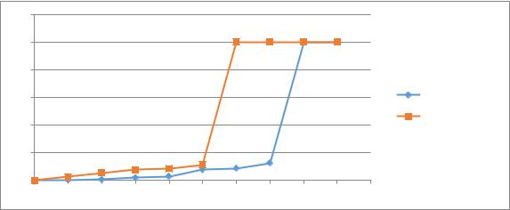
13
рый декодер по надежностям UMP, практически приближаясь к вероятности ошибки, получаемой при вероятностном декодировании кодов с низкой плотностью проверок на четность. Помимо независимости от характеристик канала многопороговый декодер обладает свойством декодеров кодов с низкой плотностью проверок на четность, а именно универсальностью и применимостью для любой конструкции таких кодов.
Следует отметить, что эффективность нерегулярных LDPC-кодов оказывается выше эффективности регулярных кодов. это объясняется тем, что в нерегулярных кодах из-за различного числа единиц в строках и столбцах информационные символы защищены по разному. В результате при декодировании проявляется так называемый эффект волны, когда более защищенные биты декодируются быстрее и затем как бы помогают при декодировании менее защищенных бит.
3 ПРАКТИЧЕСКАЯ ЧАСТЬ
Задание на лабораторную работу:
1.Изучить работу приложения «LDPC Кодер-Декодер»;
2.Установить параметры матрицы, выставив значения n=100, m=50, j=3, Message Bits = 1000;
3.Меняя значение параметра Noise выписать показания контроллеров BER с использованием кодирования и без него
4.По полученным данным построить соответствующие графики.
5.Привести рисунки, демонстрирующие исходное сообщение, закодированное сообщение, декодированное сообщение и разницу между исходным
идекодированным сообщением.
|
1,2 |
||||||||||
|
1 |
||||||||||
|
0,8 |
||||||||||
|
0,6 |
BER(Coding) |
|||||||||
|
0,4 |
BER(No Coding) |
|||||||||
|
0,2 |
||||||||||
|
0 |
||||||||||
|
0 |
0,02 |
0,04 |
0,06 |
0,08 |
0,1 |
0,12 |
0,14 |
0,16 |
0,18 |
0,2 |
Рис. 3 — График зависимости BER от Noise
На данном графике видно, что быстрее единицы достиг счётчик, который считал BER в канале без кодирования LDPC.

14
Виртуальная лаборатория LabVIEW — LDPC кодирование
Рис. 4 — Панель управления аппаратно-программного комплекса LDPC кодера-декодера
Рис. 5 — Исходное сообщение
Рис. 6 — Закодированное сообщение
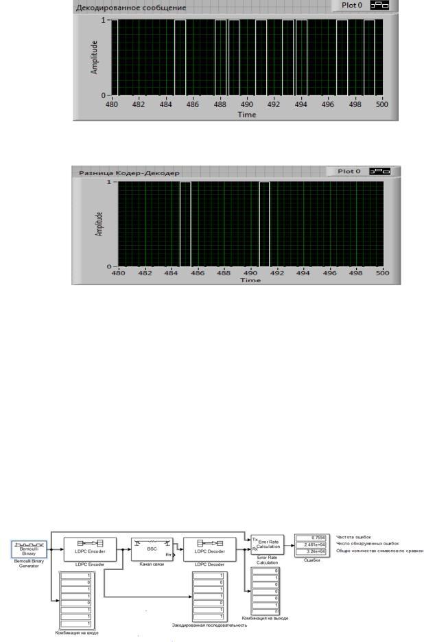
15
Рис. 7 — Декодированное сообщение
Рис. 8 — Разница между исходным и декодированным сообщением
В ходе данной лабораторной работы были закреплены навыки работы с ПО LabVIEW, изучен учебный аппаратно-программный комплекс для визуализации и исследования методов канального кодирования/декодирования в беспроводных системах цифрового вещания и связи. Данный комплекс позволяет проводить исследование кодов LDPC. Были сделаны выводы о том, что в канале с кодированием LDPC стопроцентная ошибка возникнет лишь при значении шума, равном 0,16. Тогда как в канале без кодирования стопроцентная ошибка достигается уже при 0,1.
Моделирование LDPC кодов в MATLAB Simulink
В рабочем поле необходимо собрать схему для работы кода LDPC. Схема представлена на рисунке 9
Рис. 9 — Линия передачи с применением код LDPC
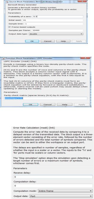
16
В состав линии с кодированием входят:
1.Bernoulli Binary Generator
2.LDPC Encoder
3.Binary Symmetric Channel (канал передачи)
4.LDPC Decoder
5.Error Rate Calculation (анализатор ошибок)
6.Display
Данные блоки необходимо найти в окне «Simulink Library». Для упрощения поиска, можно воспользоваться окошком поиска элементов.
Характеристики блоков выставить следующие:
Рис. 10 — Bernoulli Binary Generator
Рис. 11 — Binary Symmetric Channel
Рис. 12 — BCH Decoder
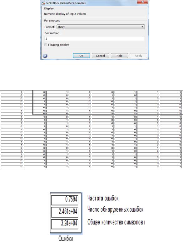
17
Рис. 13 — Error Rate Calculation (анализатор ошибок)
Представим полученные результаты:
Рис. 14 — Комбинация на входе
Рис. 15 — Работа блока оценки ошибки в канале

|
18 |
||||||||||
|
1,2 |
||||||||||
|
1 |
||||||||||
|
0,8 |
||||||||||
|
0,6 |
BER(Coding) |
|||||||||
|
BER(No Coding) |
||||||||||
|
0,4 |
||||||||||
|
0,2 |
||||||||||
|
0 |
||||||||||
|
0 |
0,02 |
0,04 |
0,06 |
0,08 |
0,1 |
0,12 |
0,14 |
0,16 |
0,18 |
0,2 |
Рис. 16 — График зависимости BER от Noise
LDPC – коды получили широкое распространение благодаря превосходной эффективности. Использование LDPC – кодов предусматривает большинство современных стандартов передачи данных (например, стандарты IEEE 802.11, IEEE 802.16), стандартов цифрового вещания (например, стандарты
DVB-S2, DVB-T2, DVB-C2).
ЛИТЕРАТУРА
1. Голиков А.М. Модуляция, кодирование и моделирование в телекоммуникационных системах. Теория и практика: Учебное пособие / А.М. Голиков. — СПб.: Издательство «Лань», 2018. – 452с.