Так как гетероскедастичность не приводит к смещению оценок коэффициентов, можно по-прежнему использовать МНК. Смещены и несостоятельны оказываются не сами оценки коэффициентов, а их стандартные ошибки, поэтому формула для расчета стандартных ошибок в условиях гомоскедастичности не подходит для случая гетероскедастичности.
Естественной идеей в этой ситуации является корректировка формулы расчета стандартных ошибок, чтобы она давала «правильный» (состоятельный) результат. Тогда можно снова будет корректно проводить тесты, проверяющие, например, незначимость коэффициентов, и строить доверительные интервалы. Соответствующие «правильные» стандартные ошибки называются состоятельными в условиях гетероскедастичности стандартными ошибками (heteroskedasticity consistent (heteroskedasticity robust) standard errors)1. Первоначальная формула для их расчета была предложена Уайтом, поэтому иногда их также называют стандартными ошибками в форме Уайта (White standard errors). Предложенная Уайтом состоятельная оценка ковариационной матрицы вектора оценок коэффициентов имеет вид:
\(\widehat{V}{\left( \widehat{\beta} \right) = n}\left( {X^{‘}X} \right)^{- 1}\left( {\frac{1}{n}{\sum\limits_{s = 1}^{n}e_{s}^{2}}x_{s}x_{s}^{‘}} \right)\left( {X^{‘}X} \right)^{- 1},\)
где \(x_{s}\) – это s-я строка матрицы регрессоров X. Легко видеть, что эта формула более громоздка, чем формула \(\widehat{V}{\left( \widehat{\beta} \right) = \left( {X^{‘}X} \right)^{- 1}}S^{2}\), которую мы вывели в третьей главе для случая гомоскедастичности. К счастью, на практике соответствующие вычисления не представляют сложности, так как возможность автоматически рассчитывать стандартные ошибки в форме Уайта реализована во всех современных эконометрических пакетах. Общепринятое обозначение для этой версии стандартных ошибок: «HC0». В работах (MacKinnon, White,1985) и (Davidson, MacKinnon, 2004) были предложены и альтернативные версии, которые обычно обозначаются в эконометрических пакетах «HC1», «HC2» и «HC3». Их расчетные формулы несколько отличаются, однако суть остается прежней: они позволяют состоятельно оценивать стандартные отклонения МНК-оценок коэффициентов в условиях гетероскедастичности.
Для случая парной регрессии состоятельная в условиях гетероскедастичности стандартная ошибка оценки коэффициента при регрессоре имеет вид:
\(\mathit{se}{\left( \widehat{\beta_{2}} \right) = \sqrt{\frac{1}{n}\frac{\frac{1}{n — 2}{\sum\limits_{i = 1}^{n}{\left( {x_{i} — \overline{x}} \right)^{2}e_{i}^{2}}}}{\widehat{\mathit{var}}(x)^{2}}.}}\)
Формальное доказательство состоятельности будет приведено в следующей главе. Пока же обсудим пример, иллюстрирующий важность использования робастных стандартных ошибок.
Пример 5.1. Оценка эффективности использования удобрений
В файле Agriculture в материалах к этому учебнику содержатся следующие данные 2010 года об урожайности яровой и озимой пшеницы в Спасском районе Пензенской области:
PRODP — урожайность в денежном выражении, в тысячах рублей с 1 га,
SIZE – размер пахотного поля, га,
LABOUR – трудозатраты, руб. на 1 га,
FUNG1 – фунгициды, протравители семян, расходы на удобрение в руб. на 1 га,
FUNG2 – фунгициды, во время роста, расходы на удобрение в руб. на 1 га,
GIRB – гербициды, расходы на удобрение в руб. на 1 га,
INSEC – инсектициды, расходы на удобрение в руб. на 1 га,
YDOB1 – аммофос, во время сева, расходы на удобрение в руб. на 1 га,
YDOB2 – аммиачная селитра, во время роста, расходы на удобрение в руб. на 1 га.
Представим, что вас интересует ответ на вопрос: влияет ли использование фунгицидов на урожайность поля?
(а) Оцените зависимость урожайности в денежном выражении от константы и переменных FUNG1, FUNG2, YDOB1, YDOB2, GIRB, INSEC, LABOUR. Запишите уравнение регрессии в стандартной форме, указав коэффициент детерминации и (в скобках под соответствующими коэффициентами) стандартные ошибки для случая гомоскедастичности. Какие из переменных значимы на 5-процентном уровне значимости?
(б) Решите предыдущий пункт заново, используя теперь состоятельные в условиях гетероскедастичности стандартные ошибки. Сопоставьте выводы по поводу значимости (при пятипроцентном уровне) переменных, характеризующих использование фунгицидов.
Решение:
(а) Оценим требуемое уравнение:
Модель 1: МНК, использованы наблюдения 1-200
Зависимая переменная: PRODP
| Коэффициент | Ст. ошибка | t-статистика | P-значение | ||
| const | -38,4019 | 7,5273 | -5,1017 | <0,00001 | *** |
| FUNG1 | 0,0445755 | 0,0487615 | 0,9142 | 0,36178 | |
| FUNG2 | 0,103625 | 0,049254 | 2,1039 | 0,03669 | ** |
| GIRB | 0,0776059 | 0,0523553 | 1,4823 | 0,13990 | |
| INSEC | 0,0782521 | 0,0484667 | 1,6146 | 0,10805 | |
| LABOUR | 0,0415064 | 0,00275277 | 15,0781 | <0,00001 | *** |
| YDOB1 | 0,0492168 | 0,0233328 | 2,1093 | 0,03621 | ** |
| YDOB2 | -0,0906824 | 0,025864 | -3,5061 | 0,00057 | *** |
| Сумма кв. остатков | 150575,6 | Ст. ошибка модели | 28,00443 | |
| R-квадрат | 0,801958 | Испр. R-квадрат | 0,794738 | |
| F(7, 192) | 111,0701 | Р-значение (F) | 5,08e-64 |
Переменные FUNG2, LABOUR, YDOB1 и YDOB2 значимы на пятипроцентном уровне значимости (причем LABOUR и YDOB2 — ещё и на однопроцентном).
Если представить те же самые результаты в форме уравнения, то получится вот так:
\({\widehat{\mathit{PRODP}}}_{i} = {{- \underset{(7,53)}{38,40}} + {\underset{(0,05)}{0,04} \ast {\mathit{FUNG}1}_{i}} + {\underset{(0,05)}{0,10} \ast {\mathit{FUNG}2}_{i}} +}\)
\({{+ \underset{(0,05)}{0,08}} \ast \mathit{GIRB}_{i}} + {\underset{(0,05)}{0,08} \ast \mathit{INSEC}_{i}} + {\underset{(0,003)}{0,04} \ast \mathit{LABOUR}_{i}} + {}\)
\({{{+ \underset{(0,02)}{0,05}} \ast {\mathit{YDOB}1}_{i}} — {\underset{(0,03)}{0,09} \ast {\mathit{YDOB}2}_{i}}},{R^{2} = 0,802}\)
(б) При использовании альтернативных стандартных ошибок получим следующий результат:
Модель 2: МНК, использованы наблюдения 1-200
Зависимая переменная: PRODP
Робастные оценки стандартных ошибок (с поправкой на гетероскедастичность),
вариант HC1
| Коэффициент | Ст. ошибка | t-статистика | P-значение | ||
| const | -38,4019 | 7,40425 | -5,1865 | <0,00001 | *** |
| FUNG1 | 0,0445755 | 0,0629524 | 0,7081 | 0,47975 | |
| FUNG2 | 0,103625 | 0,0624082 | 1,6604 | 0,09846 | * |
| GIRB | 0,0776059 | 0,0623777 | 1,2441 | 0,21497 | |
| INSEC | 0,0782521 | 0,0536527 | 1,4585 | 0,14634 | |
| LABOUR | 0,0415064 | 0,00300121 | 13,8299 | <0,00001 | *** |
| YDOB1 | 0,0492168 | 0,0197491 | 2,4921 | 0,01355 | ** |
| YDOB2 | -0,0906824 | 0,030999 | -2,9253 | 0,00386 | *** |
| Сумма кв. остатков | 150575,6 | Ст. ошибка модели | 28,00443 | |
| R-квадрат | 0,801958 | Испр. R-квадрат | 0,794738 | |
| F(7, 192) | 119,2263 | Р-значение (F) | 2,16e-66 |
Оценки коэффициентов по сравнению с пунктом (а) не поменялись, что естественно: мы ведь по-прежнему используем обычный МНК. Однако стандартные ошибки теперь немного другие. В некоторых случаях это меняет выводы тестов на незначимость.
Переменные LABOUR, YDOB1 и YDOB2 значимы на пятипроцентном уровне значимости (причем LABOUR и YDOB2 — ещё и на однопроцентном).
Переменная FUNG2 перестала быть значимой на пятипроцентном уровне. Таким образом, при использовании корректных стандартных ошибок следует сделать вывод о том, что соответствующий вид удобрений не важен для урожайности. Обратите внимание, что если бы мы использовали «обычные» стандартные ошибки, то мы пришли бы к противоположному заключению (см. пункт (а)).
* * *
Важно подчеркнуть, что в реальных пространственных данных гетероскедастичность в той или иной степени наблюдается практически всегда. А даже если её и нет, то состоятельные в условиях гетероскедастичности стандартные ошибки по-прежнему будут… состоятельными (и будут близки к «обычным» стандартным ошибкам, посчитанным по формулам из третьей главы). Поэтому в современных прикладных исследованиях при оценке уравнений по умолчанию используются именно робастные стандартные ошибки, а не стандартные ошибки для случая гомоскедастичности. Мы настоятельно рекомендуем читателю поступать так же2. В нашем учебнике с этого момента и во всех последующих главах, если прямо не оговорено иное, для МНК-оценок параметров всегда используются состоятельные в условиях гетероскедастичности стандартные ошибки.
-
Поскольку довольно утомительно каждый раз произносить это название полностью в англоязычном варианте их часто называют просто robust standard errors, что на русском языке эконометристов превратилось в «робастные стандартные ошибки». Кому-то подобный англицизм, конечно, режет слух, однако в устной речи он и правда куда удобней своей длинной альтернативы.↩︎
-
Просто не забывайте включать соответствующую опцию в своем эконометрическом пакете.↩︎
Так как гетероскедастичность не приводит к смещению оценок коэффициентов, можно по-прежнему использовать МНК. Смещены и несостоятельны оказываются не сами оценки коэффициентов, а их стандартные ошибки, поэтому формула для расчета стандартных ошибок в условиях гомоскедастичности не подходит для случая гетероскедастичности.
Естественной идеей в этой ситуации является корректировка формулы расчета стандартных ошибок, чтобы она давала «правильный» (состоятельный) результат. Тогда можно снова будет корректно проводить тесты, проверяющие, например, незначимость коэффициентов, и строить доверительные интервалы. Соответствующие «правильные» стандартные ошибки называются состоятельными в условиях гетероскедастичности стандартными ошибками (heteroskedasticity consistent (heteroskedasticity robust) standard errors)1. Первоначальная формула для их расчета была предложена Уайтом, поэтому иногда их также называют стандартными ошибками в форме Уайта (White standard errors). Предложенная Уайтом состоятельная оценка ковариационной матрицы вектора оценок коэффициентов имеет вид:
(widehat{V}{left( widehat{beta} right) = n}left( {X^{‘}X} right)^{- 1}left( {frac{1}{n}{sumlimits_{s = 1}^{n}e_{s}^{2}}x_{s}x_{s}^{‘}} right)left( {X^{‘}X} right)^{- 1},)
где (x_{s}) – это s-я строка матрицы регрессоров X. Легко видеть, что эта формула более громоздка, чем формула (widehat{V}{left( widehat{beta} right) = left( {X^{‘}X} right)^{- 1}}S^{2}), которую мы вывели в третьей главе для случая гомоскедастичности. К счастью, на практике соответствующие вычисления не представляют сложности, так как возможность автоматически рассчитывать стандартные ошибки в форме Уайта реализована во всех современных эконометрических пакетах. Общепринятое обозначение для этой версии стандартных ошибок: «HC0». В работах (MacKinnon, White,1985) и (Davidson, MacKinnon, 2004) были предложены и альтернативные версии, которые обычно обозначаются в эконометрических пакетах «HC1», «HC2» и «HC3». Их расчетные формулы несколько отличаются, однако суть остается прежней: они позволяют состоятельно оценивать стандартные отклонения МНК-оценок коэффициентов в условиях гетероскедастичности.
Для случая парной регрессии состоятельная в условиях гетероскедастичности стандартная ошибка оценки коэффициента при регрессоре имеет вид:
(mathit{se}{left( widehat{beta_{2}} right) = sqrt{frac{1}{n}frac{frac{1}{n — 2}{sumlimits_{i = 1}^{n}{left( {x_{i} — overline{x}} right)^{2}e_{i}^{2}}}}{widehat{mathit{var}}(x)^{2}}.}})
Формальное доказательство состоятельности будет приведено в следующей главе. Пока же обсудим пример, иллюстрирующий важность использования робастных стандартных ошибок.
Пример 5.1. Оценка эффективности использования удобрений
В файле Agriculture в материалах к этому учебнику содержатся следующие данные 2010 года об урожайности яровой и озимой пшеницы в Спасском районе Пензенской области:
PRODP — урожайность в денежном выражении, в тысячах рублей с 1 га,
SIZE – размер пахотного поля, га,
LABOUR – трудозатраты, руб. на 1 га,
FUNG1 – фунгициды, протравители семян, расходы на удобрение в руб. на 1 га,
FUNG2 – фунгициды, во время роста, расходы на удобрение в руб. на 1 га,
GIRB – гербициды, расходы на удобрение в руб. на 1 га,
INSEC – инсектициды, расходы на удобрение в руб. на 1 га,
YDOB1 – аммофос, во время сева, расходы на удобрение в руб. на 1 га,
YDOB2 – аммиачная селитра, во время роста, расходы на удобрение в руб. на 1 га.
Представим, что вас интересует ответ на вопрос: влияет ли использование фунгицидов на урожайность поля?
(а) Оцените зависимость урожайности в денежном выражении от константы и переменных FUNG1, FUNG2, YDOB1, YDOB2, GIRB, INSEC, LABOUR. Запишите уравнение регрессии в стандартной форме, указав коэффициент детерминации и (в скобках под соответствующими коэффициентами) стандартные ошибки для случая гомоскедастичности. Какие из переменных значимы на 5-процентном уровне значимости?
(б) Решите предыдущий пункт заново, используя теперь состоятельные в условиях гетероскедастичности стандартные ошибки. Сопоставьте выводы по поводу значимости (при пятипроцентном уровне) переменных, характеризующих использование фунгицидов.
Решение:
(а) Оценим требуемое уравнение:
Модель 1: МНК, использованы наблюдения 1-200
Зависимая переменная: PRODP
| Коэффициент | Ст. ошибка | t-статистика | P-значение | ||
| const | -38,4019 | 7,5273 | -5,1017 | <0,00001 | *** |
| FUNG1 | 0,0445755 | 0,0487615 | 0,9142 | 0,36178 | |
| FUNG2 | 0,103625 | 0,049254 | 2,1039 | 0,03669 | ** |
| GIRB | 0,0776059 | 0,0523553 | 1,4823 | 0,13990 | |
| INSEC | 0,0782521 | 0,0484667 | 1,6146 | 0,10805 | |
| LABOUR | 0,0415064 | 0,00275277 | 15,0781 | <0,00001 | *** |
| YDOB1 | 0,0492168 | 0,0233328 | 2,1093 | 0,03621 | ** |
| YDOB2 | -0,0906824 | 0,025864 | -3,5061 | 0,00057 | *** |
| Сумма кв. остатков | 150575,6 | Ст. ошибка модели | 28,00443 | |
| R-квадрат | 0,801958 | Испр. R-квадрат | 0,794738 | |
| F(7, 192) | 111,0701 | Р-значение (F) | 5,08e-64 |
Переменные FUNG2, LABOUR, YDOB1 и YDOB2 значимы на пятипроцентном уровне значимости (причем LABOUR и YDOB2 — ещё и на однопроцентном).
Если представить те же самые результаты в форме уравнения, то получится вот так:
({widehat{mathit{PRODP}}}_{i} = {{- underset{(7,53)}{38,40}} + {underset{(0,05)}{0,04} ast {mathit{FUNG}1}_{i}} + {underset{(0,05)}{0,10} ast {mathit{FUNG}2}_{i}} +})
({{+ underset{(0,05)}{0,08}} ast mathit{GIRB}_{i}} + {underset{(0,05)}{0,08} ast mathit{INSEC}_{i}} + {underset{(0,003)}{0,04} ast mathit{LABOUR}_{i}} + {})
({{{+ underset{(0,02)}{0,05}} ast {mathit{YDOB}1}_{i}} — {underset{(0,03)}{0,09} ast {mathit{YDOB}2}_{i}}},{R^{2} = 0,802})
(б) При использовании альтернативных стандартных ошибок получим следующий результат:
Модель 2: МНК, использованы наблюдения 1-200
Зависимая переменная: PRODP
Робастные оценки стандартных ошибок (с поправкой на гетероскедастичность),
вариант HC1
| Коэффициент | Ст. ошибка | t-статистика | P-значение | ||
| const | -38,4019 | 7,40425 | -5,1865 | <0,00001 | *** |
| FUNG1 | 0,0445755 | 0,0629524 | 0,7081 | 0,47975 | |
| FUNG2 | 0,103625 | 0,0624082 | 1,6604 | 0,09846 | * |
| GIRB | 0,0776059 | 0,0623777 | 1,2441 | 0,21497 | |
| INSEC | 0,0782521 | 0,0536527 | 1,4585 | 0,14634 | |
| LABOUR | 0,0415064 | 0,00300121 | 13,8299 | <0,00001 | *** |
| YDOB1 | 0,0492168 | 0,0197491 | 2,4921 | 0,01355 | ** |
| YDOB2 | -0,0906824 | 0,030999 | -2,9253 | 0,00386 | *** |
| Сумма кв. остатков | 150575,6 | Ст. ошибка модели | 28,00443 | |
| R-квадрат | 0,801958 | Испр. R-квадрат | 0,794738 | |
| F(7, 192) | 119,2263 | Р-значение (F) | 2,16e-66 |
Оценки коэффициентов по сравнению с пунктом (а) не поменялись, что естественно: мы ведь по-прежнему используем обычный МНК. Однако стандартные ошибки теперь немного другие. В некоторых случаях это меняет выводы тестов на незначимость.
Переменные LABOUR, YDOB1 и YDOB2 значимы на пятипроцентном уровне значимости (причем LABOUR и YDOB2 — ещё и на однопроцентном).
Переменная FUNG2 перестала быть значимой на пятипроцентном уровне. Таким образом, при использовании корректных стандартных ошибок следует сделать вывод о том, что соответствующий вид удобрений не важен для урожайности. Обратите внимание, что если бы мы использовали «обычные» стандартные ошибки, то мы пришли бы к противоположному заключению (см. пункт (а)).
* * *
Важно подчеркнуть, что в реальных пространственных данных гетероскедастичность в той или иной степени наблюдается практически всегда. А даже если её и нет, то состоятельные в условиях гетероскедастичности стандартные ошибки по-прежнему будут… состоятельными (и будут близки к «обычным» стандартным ошибкам, посчитанным по формулам из третьей главы). Поэтому в современных прикладных исследованиях при оценке уравнений по умолчанию используются именно робастные стандартные ошибки, а не стандартные ошибки для случая гомоскедастичности. Мы настоятельно рекомендуем читателю поступать так же2. В нашем учебнике с этого момента и во всех последующих главах, если прямо не оговорено иное, для МНК-оценок параметров всегда используются состоятельные в условиях гетероскедастичности стандартные ошибки.
-
Поскольку довольно утомительно каждый раз произносить это название полностью в англоязычном варианте их часто называют просто robust standard errors, что на русском языке эконометристов превратилось в «робастные стандартные ошибки». Кому-то подобный англицизм, конечно, режет слух, однако в устной речи он и правда куда удобней своей длинной альтернативы.↩︎
-
Просто не забывайте включать соответствующую опцию в своем эконометрическом пакете.↩︎
Robust statistics are statistics with good performance for data drawn from a wide range of probability distributions, especially for distributions that are not normal. Robust statistical methods have been developed for many common problems, such as estimating location, scale, and regression parameters. One motivation is to produce statistical methods that are not unduly affected by outliers. Another motivation is to provide methods with good performance when there are small departures from a parametric distribution. For example, robust methods work well for mixtures of two normal distributions with different standard deviations; under this model, non-robust methods like a t-test work poorly.
Introduction[edit]
Robust statistics seek to provide methods that emulate popular statistical methods, but which are not unduly affected by outliers or other small departures from model assumptions. In statistics, classical estimation methods rely heavily on assumptions which are often not met in practice. In particular, it is often assumed that the data errors are normally distributed, at least approximately, or that the central limit theorem can be relied on to produce normally distributed estimates. Unfortunately, when there are outliers in the data, classical estimators often have very poor performance, when judged using the breakdown point and the influence function, described below.
The practical effect of problems seen in the influence function can be studied empirically by examining the sampling distribution of proposed estimators under a mixture model, where one mixes in a small amount (1–5% is often sufficient) of contamination. For instance, one may use a mixture of 95% a normal distribution, and 5% a normal distribution with the same mean but significantly higher standard deviation (representing outliers).
Robust parametric statistics can proceed in two ways:
- by designing estimators so that a pre-selected behaviour of the influence function is achieved
- by replacing estimators that are optimal under the assumption of a normal distribution with estimators that are optimal for, or at least derived for, other distributions: for example using the t-distribution with low degrees of freedom (high kurtosis; degrees of freedom between 4 and 6 have often been found to be useful in practice[citation needed]) or with a mixture of two or more distributions.
Robust estimates have been studied for the following problems:
- estimating location parameters[citation needed]
- estimating scale parameters[citation needed]
- estimating regression coefficients[citation needed]
- estimation of model-states in models expressed in state-space form, for which the standard method is equivalent to a Kalman filter.
Definition[edit]
|
This section needs expansion. You can help by adding to it. (July 2008) |
There are various definitions of a «robust statistic.» Strictly speaking, a robust statistic is resistant to errors in the results, produced by deviations from assumptions[1] (e.g., of normality). This means that if the assumptions are only approximately met, the robust estimator will still have a reasonable efficiency, and reasonably small bias, as well as being asymptotically unbiased, meaning having a bias tending towards 0 as the sample size tends towards infinity.
Usually the most important case is distributional robustness — robustness to breaking of the assumptions about the underlying distribution of the data.[1] Classical statistical procedures are typically sensitive to «longtailedness» (e.g., when the distribution of the data has longer tails than the assumed normal distribution). This implies that they will be strongly affected by the presence of outliers in the data, and the estimates they produce may be heavily distorted if there are extreme outliers in the data, compared to what they would be if the outliers were not included in the data.
By contrast, more robust estimators that are not so sensitive to distributional distortions such as longtailedness are also resistant to the presence of outliers. Thus, in the context of robust statistics, distributionally robust and outlier-resistant are effectively synonymous.[1] For one perspective on research in robust statistics up to 2000, see Portnoy & He (2000).
Some experts prefer the term resistant statistics for distributional robustness, and reserve ‘robustness’ for non-distributional robustness, e.g., robustness to violation of assumptions about the probability model or estimator, but this is a minority usage. Plain ‘robustness’ to mean ‘distributional robustness’ is common.
When considering how robust an estimator is to the presence of outliers, it is useful to test what happens when an extreme outlier is added to the dataset, and to test what happens when an extreme outlier replaces one of the existing datapoints, and then to consider the effect of multiple additions or replacements.
Examples[edit]
The mean is not a robust measure of central tendency. If the dataset is e.g. the values {2,3,5,6,9}, then if we add another datapoint with value -1000 or +1000 to the data, the resulting mean will be very different to the mean of the original data. Similarly, if we replace one of the values with a datapoint of value -1000 or +1000 then the resulting mean will be very different to the mean of the original data.
The median is a robust measure of central tendency. Taking the same dataset {2,3,5,6,9}, if we add another datapoint with value -1000 or +1000 then the median will change slightly, but it will still be similar to the median of the original data. If we replace one of the values with a datapoint of value -1000 or +1000 then the resulting median will still be similar to the median of the original data.
Described in terms of breakdown points, the median has a breakdown point of 50%, meaning that half the points must be outliers before the median can be moved outside the range of the non-outliers, while the mean has a breakdown point of 0, as a single large observation can throw it off.
The median absolute deviation and interquartile range are robust measures of statistical dispersion, while the standard deviation and range are not.
Trimmed estimators and Winsorised estimators are general methods to make statistics more robust. L-estimators are a general class of simple statistics, often robust, while M-estimators are a general class of robust statistics, and are now the preferred solution, though they can be quite involved to calculate.
Speed-of-light data[edit]
Gelman et al. in Bayesian Data Analysis (2004) consider a data set relating to speed-of-light measurements made by Simon Newcomb. The data sets for that book can be found via the Classic data sets page, and the book’s website contains more information on the data.
Although the bulk of the data look to be more or less normally distributed, there are two obvious outliers. These outliers have a large effect on the mean, dragging it towards them, and away from the center of the bulk of the data. Thus, if the mean is intended as a measure of the location of the center of the data, it is, in a sense, biased when outliers are present.
Also, the distribution of the mean is known to be asymptotically normal due to the central limit theorem. However, outliers can make the distribution of the mean non-normal even for fairly large data sets. Besides this non-normality, the mean is also inefficient in the presence of outliers and less variable measures of location are available.
Estimation of location[edit]
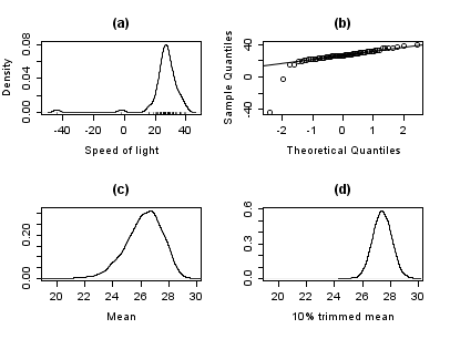
The plot below shows a density plot of the speed-of-light data, together with a rug plot (panel (a)). Also shown is a normal Q–Q plot (panel (b)). The outliers are clearly visible in these plots.
Panels (c) and (d) of the plot show the bootstrap distribution of the mean (c) and the 10% trimmed mean (d). The trimmed mean is a simple robust estimator of location that deletes a certain percentage of observations (10% here) from each end of the data, then computes the mean in the usual way. The analysis was performed in R and 10,000 bootstrap samples were used for each of the raw and trimmed means.
The distribution of the mean is clearly much wider than that of the 10% trimmed mean (the plots are on the same scale). Also whereas the distribution of the trimmed mean appears to be close to normal, the distribution of the raw mean is quite skewed to the left. So, in this sample of 66 observations, only 2 outliers cause the central limit theorem to be inapplicable.
Robust statistical methods, of which the trimmed mean is a simple example, seek to outperform classical statistical methods in the presence of outliers, or, more generally, when underlying parametric assumptions are not quite correct.
Whilst the trimmed mean performs well relative to the mean in this example, better robust estimates are available. In fact, the mean, median and trimmed mean are all special cases of M-estimators. Details appear in the sections below.
Estimation of scale[edit]
The outliers in the speed-of-light data have more than just an adverse effect on the mean; the usual estimate of scale is the standard deviation, and this quantity is even more badly affected by outliers because the squares of the deviations from the mean go into the calculation, so the outliers’ effects are exacerbated.
The plots below show the bootstrap distributions of the standard deviation, the median absolute deviation (MAD) and the Rousseeuw–Croux (Qn) estimator of scale.[2] The plots are based on 10,000 bootstrap samples for each estimator, with some Gaussian noise added to the resampled data (smoothed bootstrap). Panel (a) shows the distribution of the standard deviation, (b) of the MAD and (c) of Qn.

The distribution of standard deviation is erratic and wide, a result of the outliers. The MAD is better behaved, and Qn is a little bit more efficient than MAD. This simple example demonstrates that when outliers are present, the standard deviation cannot be recommended as an estimate of scale.
Manual screening for outliers[edit]
Traditionally, statisticians would manually screen data for outliers, and remove them, usually checking the source of the data to see whether the outliers were erroneously recorded. Indeed, in the speed-of-light example above, it is easy to see and remove the two outliers prior to proceeding with any further analysis. However, in modern times, data sets often consist of large numbers of variables being measured on large numbers of experimental units. Therefore, manual screening for outliers is often impractical.
Outliers can often interact in such a way that they mask each other. As a simple example, consider a small univariate data set containing one modest and one large outlier. The estimated standard deviation will be grossly inflated by the large outlier. The result is that the modest outlier looks relatively normal. As soon as the large outlier is removed, the estimated standard deviation shrinks, and the modest outlier now looks unusual.
This problem of masking gets worse as the complexity of the data increases. For example, in regression problems, diagnostic plots are used to identify outliers. However, it is common that once a few outliers have been removed, others become visible. The problem is even worse in higher dimensions.
Robust methods provide automatic ways of detecting, downweighting (or removing), and flagging outliers, largely removing the need for manual screening. Care must be taken; initial data showing the ozone hole first appearing over Antarctica were rejected as outliers by non-human screening.[3]
Variety of applications[edit]
Although this article deals with general principles for univariate statistical methods, robust methods also exist for regression problems, generalized linear models, and parameter estimation of various distributions.
Measures of robustness[edit]
The basic tools used to describe and measure robustness are, the breakdown point, the influence function and the sensitivity curve.
Breakdown point[edit]
Intuitively, the breakdown point of an estimator is the proportion of incorrect observations (e.g. arbitrarily large observations) an estimator can handle before giving an incorrect (e.g., arbitrarily large) result. Usually the asymptotic (infinite sample) limit is quoted as the breakdown point, although the finite-sample breakdown point may be more useful.[4] For example, given  independent random variables
  and the corresponding realizations
  , we can use
  to estimate the mean. Such an estimator has a breakdown point of 0 (or finite-sample breakdown point of
  ) because we can make
  arbitrarily large just by changing any of .
The higher the breakdown point of an estimator, the more robust it is. Intuitively, we can understand that a breakdown point cannot exceed 50% because if more than half of the observations are contaminated, it is not possible to distinguish between the underlying distribution and the contaminating distribution Rousseeuw & Leroy (1986). Therefore, the maximum breakdown point is 0.5 and there are estimators which achieve such a breakdown point. For example, the median has a breakdown point of 0.5. The X% trimmed mean has breakdown point of X%, for the chosen level of X. Huber (1981) and Maronna, Martin & Yohai (2006) contain more details. The level and the power breakdown points of tests are investigated in He, Simpson & Portnoy (1990).
Statistics with high breakdown points are sometimes called resistant statistics.[5]
Example: speed-of-light data[edit]
In the speed-of-light example, removing the two lowest observations causes the mean to change from 26.2 to 27.75, a change of 1.55. The estimate of scale produced by the Qn method is 6.3. We can divide this by the square root of the sample size to get a robust standard error, and we find this quantity to be 0.78. Thus, the change in the mean resulting from removing two outliers is approximately twice the robust standard error.
The 10% trimmed mean for the speed-of-light data is 27.43. Removing the two lowest observations and recomputing gives 27.67. Clearly, the trimmed mean is less affected by the outliers and has a higher breakdown point.
If we replace the lowest observation, −44, by −1000, the mean becomes 11.73, whereas the 10% trimmed mean is still 27.43. In many areas of applied statistics, it is common for data to be log-transformed to make them near symmetrical. Very small values become large negative when log-transformed, and zeroes become negatively infinite. Therefore, this example is of practical interest.
Empirical influence function[edit]
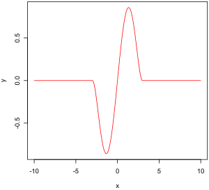
Tukey’s biweight function
The empirical influence function is a measure of the dependence of the estimator on the value of any one of the points in the sample. It is a model-free measure in the sense that it simply relies on calculating the estimator again with a different sample. On the right is Tukey’s biweight function, which, as we will later see, is an example of what a «good» (in a sense defined later on) empirical influence function should look like.
In mathematical terms, an influence function is defined as a vector in the space of the estimator, which is in turn defined for a sample which is a subset of the population:
 is a probability space,
- is a measurable space (state space),
- is a parameter space of dimension ,
- is a measurable space,


For example,
- is any probability space,
- ,
- ,


The empirical influence function is defined as follows.
Let  and
and  are i.i.d. and
  is a sample from these variables.
  is an estimator. Let
  . The empirical influence function
  at observation
  is defined by:

What this actually means is that we are replacing the i-th value in the sample by an arbitrary value and looking at the output of the estimator. Alternatively, the EIF is defined as the effect, scaled by n+1 instead of n, on the estimator of adding the point  to the sample.[citation needed]
Influence function and sensitivity curve[edit]
Instead of relying solely on the data, we could use the distribution of the random variables. The approach is quite different from that of the previous paragraph. What we are now trying to do is to see what happens to an estimator when we change the distribution of the data slightly: it assumes a distribution, and measures sensitivity to change in this distribution. By contrast, the empirical influence assumes a sample set, and measures sensitivity to change in the samples.[6]
Let  be a convex subset of the set of all finite signed measures on
  . We want to estimate the parameter
  of a distribution
  in . Let the functional
  be the asymptotic value of some estimator sequence
  . We will suppose that this functional is Fisher consistent, i.e.
  . This means that at the model , the estimator sequence asymptotically measures the correct quantity.
Let  be some distribution in . What happens when the data doesn’t follow the model exactly but another, slightly different, «going towards» ?
We’re looking at:  ,
,
which is the one-sided Gateaux derivative of  at , in the direction of
  .
.
Let  .
.  is the probability measure which gives mass 1 to
  . We choose
  . The influence function is then defined by:

It describes the effect of an infinitesimal contamination at the point on the estimate we are seeking, standardized by the mass  of the contamination (the asymptotic bias caused by contamination in the observations). For a robust estimator, we want a bounded influence function, that is, one which does not go to infinity as x becomes arbitrarily large.
Desirable properties[edit]
Properties of an influence function which bestow it with desirable performance are:
- Finite rejection point ,
- Small gross-error sensitivity ,
- Small local-shift sensitivity .


Rejection point[edit]

Gross-error sensitivity[edit]

Local-shift sensitivity[edit]

This value, which looks a lot like a Lipschitz constant, represents the effect of shifting an observation slightly from to a neighbouring point  , i.e., add an observation at and remove one at .
M-estimators[edit]
(The mathematical context of this paragraph is given in the section on empirical influence functions.)
Historically, several approaches to robust estimation were proposed, including R-estimators and L-estimators. However, M-estimators now appear to dominate the field as a result of their generality, high breakdown point, and their efficiency. See Huber (1981).
M-estimators are a generalization of maximum likelihood estimators (MLEs). What we try to do with MLE’s is to maximize  or, equivalently, minimize
  . In 1964, Huber proposed to generalize this to the minimization of
  , where
  is some function. MLE are therefore a special case of M-estimators (hence the name: «Maximum likelihood type» estimators).
Minimizing can often be done by differentiating and solving  , where
  (if has a derivative).
Several choices of and  have been proposed. The two figures below show four functions and their corresponding functions.

For squared errors,  increases at an accelerating rate, whilst for absolute errors, it increases at a constant rate. When Winsorizing is used, a mixture of these two effects is introduced: for small values of x, increases at the squared rate, but once the chosen threshold is reached (1.5 in this example), the rate of increase becomes constant. This Winsorised estimator is also known as the Huber loss function.
Tukey’s biweight (also known as bisquare) function behaves in a similar way to the squared error function at first, but for larger errors, the function tapers off.

Properties of M-estimators[edit]
M-estimators do not necessarily relate to a probability density function. Therefore, off-the-shelf approaches to inference that arise from likelihood theory can not, in general, be used.
It can be shown that M-estimators are asymptotically normally distributed, so that as long as their standard errors can be computed, an approximate approach to inference is available.
Since M-estimators are normal only asymptotically, for small sample sizes it might be appropriate to use an alternative approach to inference, such as the bootstrap. However, M-estimates are not necessarily unique (i.e., there might be more than one solution that satisfies the equations). Also, it is possible that any particular bootstrap sample can contain more outliers than the estimator’s breakdown point. Therefore, some care is needed when designing bootstrap schemes.
Of course, as we saw with the speed-of-light example, the mean is only normally distributed asymptotically and when outliers are present the approximation can be very poor even for quite large samples. However, classical statistical tests, including those based on the mean, are typically bounded above by the nominal size of the test. The same is not true of M-estimators and the type I error rate can be substantially above the nominal level.
These considerations do not «invalidate» M-estimation in any way. They merely make clear that some care is needed in their use, as is true of any other method of estimation.
Influence function of an M-estimator[edit]
It can be shown that the influence function of an M-estimator is proportional to ,[7] which means we can derive the properties of such an estimator (such as its rejection point, gross-error sensitivity or local-shift sensitivity) when we know its function.

with the  given by:

Choice of ψ and ρ[edit]
In many practical situations, the choice of the function is not critical to gaining a good robust estimate, and many choices will give similar results that offer great improvements, in terms of efficiency and bias, over classical estimates in the presence of outliers.[8]
Theoretically, functions are to be preferred,[clarification needed] and Tukey’s biweight (also known as bisquare) function is a popular choice. Maronna, Martin & Yohai (2006) recommend the biweight function with efficiency at the normal set to 85%.
Robust parametric approaches[edit]
M-estimators do not necessarily relate to a density function and so are not fully parametric. Fully parametric approaches to robust modeling and inference, both Bayesian and likelihood approaches, usually deal with heavy tailed distributions such as Student’s t-distribution.
For the t-distribution with  degrees of freedom, it can be shown that

For  , the t-distribution is equivalent to the Cauchy distribution. The degrees of freedom is sometimes known as the kurtosis parameter. It is the parameter that controls how heavy the tails are. In principle, can be estimated from the data in the same way as any other parameter. In practice, it is common for there to be multiple local maxima when is allowed to vary. As such, it is common to fix at a value around 4 or 6. The figure below displays the -function for 4 different values of .

Example: speed-of-light data[edit]
For the speed-of-light data, allowing the kurtosis parameter to vary and maximizing the likelihood, we get

Fixing  and maximizing the likelihood gives

[edit]
A pivotal quantity is a function of data, whose underlying population distribution is a member of a parametric family, that is not dependent on the values of the parameters. An ancillary statistic is such a function that is also a statistic, meaning that it is computed in terms of the data alone. Such functions are robust to parameters in the sense that they are independent of the values of the parameters, but not robust to the model in the sense that they assume an underlying model (parametric family), and in fact such functions are often very sensitive to violations of the model assumptions. Thus test statistics, frequently constructed in terms of these to not be sensitive to assumptions about parameters, are still very sensitive to model assumptions.
Replacing outliers and missing values[edit]
Replacing missing data is called imputation. If there are relatively few missing points, there are some models which can be used to estimate values to complete the series, such as replacing missing values with the mean or median of the data. Simple linear regression can also be used to estimate missing values.[9][incomplete short citation] In addition, outliers can sometimes be accommodated in the data through the use of trimmed means, other scale estimators apart from standard deviation (e.g., MAD) and Winsorization.[10] In calculations of a trimmed mean, a fixed percentage of data is dropped from each end of an ordered data, thus eliminating the outliers. The mean is then calculated using the remaining data. Winsorizing involves accommodating an outlier by replacing it with the next highest or next smallest value as appropriate.[11]
However, using these types of models to predict missing values or outliers in a long time series is difficult and often unreliable, particularly if the number of values to be in-filled is relatively high in comparison with total record length. The accuracy of the estimate depends on how good and representative the model is and how long the period of missing values extends.[12] When dynamic evolution is assumed in a series, the missing data point problem becomes an exercise in multivariate analysis (rather than the univariate approach of most traditional methods of estimating missing values and outliers). In such cases, a multivariate model will be more representative than a univariate one for predicting missing values. The Kohonen self organising map (KSOM) offers a simple and robust multivariate model for data analysis, thus providing good possibilities to estimate missing values, taking into account its relationship or correlation with other pertinent variables in the data record.[11]
Standard Kalman filters are not robust to outliers. To this end Ting, Theodorou & Schaal (2007) have recently shown that a modification of Masreliez’s theorem can deal with outliers.
One common approach to handle outliers in data analysis is to perform outlier detection first, followed by an efficient estimation method (e.g., the least squares). While this approach is often useful, one must keep in mind two challenges. First, an outlier detection method that relies on a non-robust initial fit can suffer from the effect of masking, that is, a group of outliers can mask each other and escape detection.[13] Second, if a high breakdown initial fit is used for outlier detection, the follow-up analysis might inherit some of the inefficiencies of the initial estimator.[14]
See also[edit]
- Robust confidence intervals
- Robust regression
- Unit-weighted regression
Notes[edit]
- ^ a b c Huber (1981), page 1.
- ^ Rousseeuw & Croux (1993).
- ^ Masters, Jeffrey. «When was the ozone hole discovered». Weather Underground. Archived from the original on 2016-09-15.
- ^ Maronna, Martin & Yohai (2006)
- ^ Resistant statistics, David B. Stephenson
- ^ von Mises (1947).
- ^ Huber (1981), page 45
- ^ Huber (1981).
- ^ MacDonald & Zucchini (1997); Harvey (1989).
- ^ McBean & Rovers (1998).
- ^ a b Rustum & Adeloye (2007).
- ^ Rosen & Lennox (2001).
- ^ Rousseeuw & Leroy (1987).
- ^ He & Portnoy (1992).
References[edit]
- Farcomeni, A.; Greco, L. (2013), Robust methods for data reduction, Boca Raton, FL: Chapman & Hall/CRC Press, ISBN 978-1-4665-9062-5.
- Hampel, Frank R.; Ronchetti, Elvezio M.; Rousseeuw, Peter J.; Stahel, Werner A. (1986), Robust statistics, Wiley Series in Probability and Mathematical Statistics: Probability and Mathematical Statistics, New York: John Wiley & Sons, Inc., ISBN 0-471-82921-8, MR 0829458. Republished in paperback, 2005.
- He, Xuming; Portnoy, Stephen (1992), «Reweighted LS estimators converge at the same rate as the initial estimator», Annals of Statistics, 20 (4): 2161–2167, doi:10.1214/aos/1176348910, MR 1193333.
- He, Xuming; Simpson, Douglas G.; Portnoy, Stephen L. (1990), «Breakdown robustness of tests», Journal of the American Statistical Association, 85 (410): 446–452, doi:10.2307/2289782, JSTOR 2289782, MR 1141746.
- Hettmansperger, T. P.; McKean, J. W. (1998), Robust nonparametric statistical methods, Kendall’s Library of Statistics, vol. 5, New York: John Wiley & Sons, Inc., ISBN 0-340-54937-8, MR 1604954. 2nd ed., CRC Press, 2011.
- Huber, Peter J. (1981), Robust statistics, New York: John Wiley & Sons, Inc., ISBN 0-471-41805-6, MR 0606374. Republished in paperback, 2004. 2nd ed., Wiley, 2009.
- Maronna, Ricardo A.; Martin, R. Douglas; Yohai, Victor J.; Salibián-Barrera, Matías (2019), Robust statistics: Theory and methods (with R), Wiley Series in Probability and Statistics (2nd ed.), Chichester: John Wiley & Sons, Ltd., doi:10.1002/9781119214656, ISBN 978-1-119-21468-7.
- McBean, Edward A.; Rovers, Frank (1998), Statistical procedures for analysis of environmental monitoring data and assessment, Prentice-Hall.
- Portnoy, Stephen; He, Xuming (2000), «A robust journey in the new millennium», Journal of the American Statistical Association, 95 (452): 1331–1335, doi:10.2307/2669782, JSTOR 2669782, MR 1825288.
- Press, William H.; Teukolsky, Saul A.; Vetterling, William T.; Flannery, Brian P. (2007), «Section 15.7. Robust Estimation», Numerical Recipes: The Art of Scientific Computing (3rd ed.), Cambridge University Press, ISBN 978-0-521-88068-8, MR 2371990.
- Rosen, C.; Lennox, J.A. (October 2001), «Multivariate and multiscale monitoring of wastewater treatment operation», Water Research, 35 (14): 3402–3410, doi:10.1016/s0043-1354(01)00069-0, PMID 11547861.
- Rousseeuw, Peter J.; Croux, Christophe (1993), «Alternatives to the median absolute deviation», Journal of the American Statistical Association, 88 (424): 1273–1283, doi:10.2307/2291267, JSTOR 2291267, MR 1245360.
- Rousseeuw, Peter J.; Leroy, Annick M. (1987), Robust Regression and Outlier Detection, Wiley Series in Probability and Mathematical Statistics: Applied Probability and Statistics, New York: John Wiley & Sons, Inc., doi:10.1002/0471725382, ISBN 0-471-85233-3, MR 0914792. Republished in paperback, 2003.
- Rousseeuw, Peter J.; Hubert, Mia (2011), «Robust statistics for outlier detection», Wiley Interdisciplinary Reviews: Data Mining and Knowledge Discovery, 1 (1): 73–79, doi:10.1002/widm.2, S2CID 17448982. Preprint
- Rustum, Rabee; Adeloye, Adebayo J. (September 2007), «Replacing outliers and missing values from activated sludge data using Kohonen self-organizing map», Journal of Environmental Engineering, 133 (9): 909–916, doi:10.1061/(asce)0733-9372(2007)133:9(909).
- Stigler, Stephen M. (2010), «The changing history of robustness», The American Statistician, 64 (4): 277–281, doi:10.1198/tast.2010.10159, MR 2758558, S2CID 10728417.
- Ting, Jo-anne; Theodorou, Evangelos; Schaal, Stefan (2007), «A Kalman filter for robust outlier detection», International Conference on Intelligent Robots and Systems – IROS, pp. 1514–1519.
- von Mises, R. (1947), «On the asymptotic distribution of differentiable statistical functions», Annals of Mathematical Statistics, 18 (3): 309–348, doi:10.1214/aoms/1177730385, MR 0022330.
- Wilcox, Rand (2012), Introduction to robust estimation and hypothesis testing, Statistical Modeling and Decision Science (3rd ed.), Amsterdam: Elsevier/Academic Press, pp. 1–22, doi:10.1016/B978-0-12-386983-8.00001-9, ISBN 978-0-12-386983-8, MR 3286430.
External links[edit]
- Brian Ripley’s robust statistics course notes.
- Nick Fieller’s course notes on Statistical Modelling and Computation contain material on robust regression.
- David Olive’s site contains course notes on robust statistics and some data sets.
- Online experiments using R and JSXGraph
Robust statistics are statistics with good performance for data drawn from a wide range of probability distributions, especially for distributions that are not normal. Robust statistical methods have been developed for many common problems, such as estimating location, scale, and regression parameters. One motivation is to produce statistical methods that are not unduly affected by outliers. Another motivation is to provide methods with good performance when there are small departures from a parametric distribution. For example, robust methods work well for mixtures of two normal distributions with different standard deviations; under this model, non-robust methods like a t-test work poorly.
Introduction[edit]
Robust statistics seek to provide methods that emulate popular statistical methods, but which are not unduly affected by outliers or other small departures from model assumptions. In statistics, classical estimation methods rely heavily on assumptions which are often not met in practice. In particular, it is often assumed that the data errors are normally distributed, at least approximately, or that the central limit theorem can be relied on to produce normally distributed estimates. Unfortunately, when there are outliers in the data, classical estimators often have very poor performance, when judged using the breakdown point and the influence function, described below.
The practical effect of problems seen in the influence function can be studied empirically by examining the sampling distribution of proposed estimators under a mixture model, where one mixes in a small amount (1–5% is often sufficient) of contamination. For instance, one may use a mixture of 95% a normal distribution, and 5% a normal distribution with the same mean but significantly higher standard deviation (representing outliers).
Robust parametric statistics can proceed in two ways:
- by designing estimators so that a pre-selected behaviour of the influence function is achieved
- by replacing estimators that are optimal under the assumption of a normal distribution with estimators that are optimal for, or at least derived for, other distributions: for example using the t-distribution with low degrees of freedom (high kurtosis; degrees of freedom between 4 and 6 have often been found to be useful in practice[citation needed]) or with a mixture of two or more distributions.
Robust estimates have been studied for the following problems:
- estimating location parameters[citation needed]
- estimating scale parameters[citation needed]
- estimating regression coefficients[citation needed]
- estimation of model-states in models expressed in state-space form, for which the standard method is equivalent to a Kalman filter.
Definition[edit]
|
This section needs expansion. You can help by adding to it. (July 2008) |
There are various definitions of a «robust statistic.» Strictly speaking, a robust statistic is resistant to errors in the results, produced by deviations from assumptions[1] (e.g., of normality). This means that if the assumptions are only approximately met, the robust estimator will still have a reasonable efficiency, and reasonably small bias, as well as being asymptotically unbiased, meaning having a bias tending towards 0 as the sample size tends towards infinity.
Usually the most important case is distributional robustness — robustness to breaking of the assumptions about the underlying distribution of the data.[1] Classical statistical procedures are typically sensitive to «longtailedness» (e.g., when the distribution of the data has longer tails than the assumed normal distribution). This implies that they will be strongly affected by the presence of outliers in the data, and the estimates they produce may be heavily distorted if there are extreme outliers in the data, compared to what they would be if the outliers were not included in the data.
By contrast, more robust estimators that are not so sensitive to distributional distortions such as longtailedness are also resistant to the presence of outliers. Thus, in the context of robust statistics, distributionally robust and outlier-resistant are effectively synonymous.[1] For one perspective on research in robust statistics up to 2000, see Portnoy & He (2000).
Some experts prefer the term resistant statistics for distributional robustness, and reserve ‘robustness’ for non-distributional robustness, e.g., robustness to violation of assumptions about the probability model or estimator, but this is a minority usage. Plain ‘robustness’ to mean ‘distributional robustness’ is common.
When considering how robust an estimator is to the presence of outliers, it is useful to test what happens when an extreme outlier is added to the dataset, and to test what happens when an extreme outlier replaces one of the existing datapoints, and then to consider the effect of multiple additions or replacements.
Examples[edit]
The mean is not a robust measure of central tendency. If the dataset is e.g. the values {2,3,5,6,9}, then if we add another datapoint with value -1000 or +1000 to the data, the resulting mean will be very different to the mean of the original data. Similarly, if we replace one of the values with a datapoint of value -1000 or +1000 then the resulting mean will be very different to the mean of the original data.
The median is a robust measure of central tendency. Taking the same dataset {2,3,5,6,9}, if we add another datapoint with value -1000 or +1000 then the median will change slightly, but it will still be similar to the median of the original data. If we replace one of the values with a datapoint of value -1000 or +1000 then the resulting median will still be similar to the median of the original data.
Described in terms of breakdown points, the median has a breakdown point of 50%, meaning that half the points must be outliers before the median can be moved outside the range of the non-outliers, while the mean has a breakdown point of 0, as a single large observation can throw it off.
The median absolute deviation and interquartile range are robust measures of statistical dispersion, while the standard deviation and range are not.
Trimmed estimators and Winsorised estimators are general methods to make statistics more robust. L-estimators are a general class of simple statistics, often robust, while M-estimators are a general class of robust statistics, and are now the preferred solution, though they can be quite involved to calculate.
Speed-of-light data[edit]
Gelman et al. in Bayesian Data Analysis (2004) consider a data set relating to speed-of-light measurements made by Simon Newcomb. The data sets for that book can be found via the Classic data sets page, and the book’s website contains more information on the data.
Although the bulk of the data look to be more or less normally distributed, there are two obvious outliers. These outliers have a large effect on the mean, dragging it towards them, and away from the center of the bulk of the data. Thus, if the mean is intended as a measure of the location of the center of the data, it is, in a sense, biased when outliers are present.
Also, the distribution of the mean is known to be asymptotically normal due to the central limit theorem. However, outliers can make the distribution of the mean non-normal even for fairly large data sets. Besides this non-normality, the mean is also inefficient in the presence of outliers and less variable measures of location are available.
Estimation of location[edit]
The plot below shows a density plot of the speed-of-light data, together with a rug plot (panel (a)). Also shown is a normal Q–Q plot (panel (b)). The outliers are clearly visible in these plots.
Panels (c) and (d) of the plot show the bootstrap distribution of the mean (c) and the 10% trimmed mean (d). The trimmed mean is a simple robust estimator of location that deletes a certain percentage of observations (10% here) from each end of the data, then computes the mean in the usual way. The analysis was performed in R and 10,000 bootstrap samples were used for each of the raw and trimmed means.
The distribution of the mean is clearly much wider than that of the 10% trimmed mean (the plots are on the same scale). Also whereas the distribution of the trimmed mean appears to be close to normal, the distribution of the raw mean is quite skewed to the left. So, in this sample of 66 observations, only 2 outliers cause the central limit theorem to be inapplicable.
Robust statistical methods, of which the trimmed mean is a simple example, seek to outperform classical statistical methods in the presence of outliers, or, more generally, when underlying parametric assumptions are not quite correct.
Whilst the trimmed mean performs well relative to the mean in this example, better robust estimates are available. In fact, the mean, median and trimmed mean are all special cases of M-estimators. Details appear in the sections below.
Estimation of scale[edit]
The outliers in the speed-of-light data have more than just an adverse effect on the mean; the usual estimate of scale is the standard deviation, and this quantity is even more badly affected by outliers because the squares of the deviations from the mean go into the calculation, so the outliers’ effects are exacerbated.
The plots below show the bootstrap distributions of the standard deviation, the median absolute deviation (MAD) and the Rousseeuw–Croux (Qn) estimator of scale.[2] The plots are based on 10,000 bootstrap samples for each estimator, with some Gaussian noise added to the resampled data (smoothed bootstrap). Panel (a) shows the distribution of the standard deviation, (b) of the MAD and (c) of Qn.
The distribution of standard deviation is erratic and wide, a result of the outliers. The MAD is better behaved, and Qn is a little bit more efficient than MAD. This simple example demonstrates that when outliers are present, the standard deviation cannot be recommended as an estimate of scale.
Manual screening for outliers[edit]
Traditionally, statisticians would manually screen data for outliers, and remove them, usually checking the source of the data to see whether the outliers were erroneously recorded. Indeed, in the speed-of-light example above, it is easy to see and remove the two outliers prior to proceeding with any further analysis. However, in modern times, data sets often consist of large numbers of variables being measured on large numbers of experimental units. Therefore, manual screening for outliers is often impractical.
Outliers can often interact in such a way that they mask each other. As a simple example, consider a small univariate data set containing one modest and one large outlier. The estimated standard deviation will be grossly inflated by the large outlier. The result is that the modest outlier looks relatively normal. As soon as the large outlier is removed, the estimated standard deviation shrinks, and the modest outlier now looks unusual.
This problem of masking gets worse as the complexity of the data increases. For example, in regression problems, diagnostic plots are used to identify outliers. However, it is common that once a few outliers have been removed, others become visible. The problem is even worse in higher dimensions.
Robust methods provide automatic ways of detecting, downweighting (or removing), and flagging outliers, largely removing the need for manual screening. Care must be taken; initial data showing the ozone hole first appearing over Antarctica were rejected as outliers by non-human screening.[3]
Variety of applications[edit]
Although this article deals with general principles for univariate statistical methods, robust methods also exist for regression problems, generalized linear models, and parameter estimation of various distributions.
Measures of robustness[edit]
The basic tools used to describe and measure robustness are, the breakdown point, the influence function and the sensitivity curve.
Breakdown point[edit]
Intuitively, the breakdown point of an estimator is the proportion of incorrect observations (e.g. arbitrarily large observations) an estimator can handle before giving an incorrect (e.g., arbitrarily large) result. Usually the asymptotic (infinite sample) limit is quoted as the breakdown point, although the finite-sample breakdown point may be more useful.[4] For example, given independent random variables and the corresponding realizations , we can use to estimate the mean. Such an estimator has a breakdown point of 0 (or finite-sample breakdown point of ) because we can make arbitrarily large just by changing any of .
The higher the breakdown point of an estimator, the more robust it is. Intuitively, we can understand that a breakdown point cannot exceed 50% because if more than half of the observations are contaminated, it is not possible to distinguish between the underlying distribution and the contaminating distribution Rousseeuw & Leroy (1986). Therefore, the maximum breakdown point is 0.5 and there are estimators which achieve such a breakdown point. For example, the median has a breakdown point of 0.5. The X% trimmed mean has breakdown point of X%, for the chosen level of X. Huber (1981) and Maronna, Martin & Yohai (2006) contain more details. The level and the power breakdown points of tests are investigated in He, Simpson & Portnoy (1990).
Statistics with high breakdown points are sometimes called resistant statistics.[5]
Example: speed-of-light data[edit]
In the speed-of-light example, removing the two lowest observations causes the mean to change from 26.2 to 27.75, a change of 1.55. The estimate of scale produced by the Qn method is 6.3. We can divide this by the square root of the sample size to get a robust standard error, and we find this quantity to be 0.78. Thus, the change in the mean resulting from removing two outliers is approximately twice the robust standard error.
The 10% trimmed mean for the speed-of-light data is 27.43. Removing the two lowest observations and recomputing gives 27.67. Clearly, the trimmed mean is less affected by the outliers and has a higher breakdown point.
If we replace the lowest observation, −44, by −1000, the mean becomes 11.73, whereas the 10% trimmed mean is still 27.43. In many areas of applied statistics, it is common for data to be log-transformed to make them near symmetrical. Very small values become large negative when log-transformed, and zeroes become negatively infinite. Therefore, this example is of practical interest.
Empirical influence function[edit]
Tukey’s biweight function
The empirical influence function is a measure of the dependence of the estimator on the value of any one of the points in the sample. It is a model-free measure in the sense that it simply relies on calculating the estimator again with a different sample. On the right is Tukey’s biweight function, which, as we will later see, is an example of what a «good» (in a sense defined later on) empirical influence function should look like.
In mathematical terms, an influence function is defined as a vector in the space of the estimator, which is in turn defined for a sample which is a subset of the population:
- is a probability space,
- is a measurable space (state space),
- is a parameter space of dimension ,
- is a measurable space,
For example,
- is any probability space,
- ,
- ,
The empirical influence function is defined as follows.
Let and are i.i.d. and is a sample from these variables. is an estimator. Let . The empirical influence function at observation is defined by:
What this actually means is that we are replacing the i-th value in the sample by an arbitrary value and looking at the output of the estimator. Alternatively, the EIF is defined as the effect, scaled by n+1 instead of n, on the estimator of adding the point to the sample.[citation needed]
Influence function and sensitivity curve[edit]
Instead of relying solely on the data, we could use the distribution of the random variables. The approach is quite different from that of the previous paragraph. What we are now trying to do is to see what happens to an estimator when we change the distribution of the data slightly: it assumes a distribution, and measures sensitivity to change in this distribution. By contrast, the empirical influence assumes a sample set, and measures sensitivity to change in the samples.[6]
Let be a convex subset of the set of all finite signed measures on . We want to estimate the parameter of a distribution in . Let the functional be the asymptotic value of some estimator sequence . We will suppose that this functional is Fisher consistent, i.e. . This means that at the model , the estimator sequence asymptotically measures the correct quantity.
Let be some distribution in . What happens when the data doesn’t follow the model exactly but another, slightly different, «going towards» ?
We’re looking at: ,
which is the one-sided Gateaux derivative of at , in the direction of .
Let . is the probability measure which gives mass 1 to . We choose . The influence function is then defined by:
It describes the effect of an infinitesimal contamination at the point on the estimate we are seeking, standardized by the mass of the contamination (the asymptotic bias caused by contamination in the observations). For a robust estimator, we want a bounded influence function, that is, one which does not go to infinity as x becomes arbitrarily large.
Desirable properties[edit]
Properties of an influence function which bestow it with desirable performance are:
- Finite rejection point ,
- Small gross-error sensitivity ,
- Small local-shift sensitivity .
Rejection point[edit]
Gross-error sensitivity[edit]
Local-shift sensitivity[edit]
This value, which looks a lot like a Lipschitz constant, represents the effect of shifting an observation slightly from to a neighbouring point , i.e., add an observation at and remove one at .
M-estimators[edit]
(The mathematical context of this paragraph is given in the section on empirical influence functions.)
Historically, several approaches to robust estimation were proposed, including R-estimators and L-estimators. However, M-estimators now appear to dominate the field as a result of their generality, high breakdown point, and their efficiency. See Huber (1981).
M-estimators are a generalization of maximum likelihood estimators (MLEs). What we try to do with MLE’s is to maximize or, equivalently, minimize . In 1964, Huber proposed to generalize this to the minimization of , where is some function. MLE are therefore a special case of M-estimators (hence the name: «Maximum likelihood type» estimators).
Minimizing can often be done by differentiating and solving , where (if has a derivative).
Several choices of and have been proposed. The two figures below show four functions and their corresponding functions.
For squared errors, increases at an accelerating rate, whilst for absolute errors, it increases at a constant rate. When Winsorizing is used, a mixture of these two effects is introduced: for small values of x, increases at the squared rate, but once the chosen threshold is reached (1.5 in this example), the rate of increase becomes constant. This Winsorised estimator is also known as the Huber loss function.
Tukey’s biweight (also known as bisquare) function behaves in a similar way to the squared error function at first, but for larger errors, the function tapers off.
Properties of M-estimators[edit]
M-estimators do not necessarily relate to a probability density function. Therefore, off-the-shelf approaches to inference that arise from likelihood theory can not, in general, be used.
It can be shown that M-estimators are asymptotically normally distributed, so that as long as their standard errors can be computed, an approximate approach to inference is available.
Since M-estimators are normal only asymptotically, for small sample sizes it might be appropriate to use an alternative approach to inference, such as the bootstrap. However, M-estimates are not necessarily unique (i.e., there might be more than one solution that satisfies the equations). Also, it is possible that any particular bootstrap sample can contain more outliers than the estimator’s breakdown point. Therefore, some care is needed when designing bootstrap schemes.
Of course, as we saw with the speed-of-light example, the mean is only normally distributed asymptotically and when outliers are present the approximation can be very poor even for quite large samples. However, classical statistical tests, including those based on the mean, are typically bounded above by the nominal size of the test. The same is not true of M-estimators and the type I error rate can be substantially above the nominal level.
These considerations do not «invalidate» M-estimation in any way. They merely make clear that some care is needed in their use, as is true of any other method of estimation.
Influence function of an M-estimator[edit]
It can be shown that the influence function of an M-estimator is proportional to ,[7] which means we can derive the properties of such an estimator (such as its rejection point, gross-error sensitivity or local-shift sensitivity) when we know its function.
with the given by:
Choice of ψ and ρ[edit]
In many practical situations, the choice of the function is not critical to gaining a good robust estimate, and many choices will give similar results that offer great improvements, in terms of efficiency and bias, over classical estimates in the presence of outliers.[8]
Theoretically, functions are to be preferred,[clarification needed] and Tukey’s biweight (also known as bisquare) function is a popular choice. Maronna, Martin & Yohai (2006) recommend the biweight function with efficiency at the normal set to 85%.
Robust parametric approaches[edit]
M-estimators do not necessarily relate to a density function and so are not fully parametric. Fully parametric approaches to robust modeling and inference, both Bayesian and likelihood approaches, usually deal with heavy tailed distributions such as Student’s t-distribution.
For the t-distribution with degrees of freedom, it can be shown that
For , the t-distribution is equivalent to the Cauchy distribution. The degrees of freedom is sometimes known as the kurtosis parameter. It is the parameter that controls how heavy the tails are. In principle, can be estimated from the data in the same way as any other parameter. In practice, it is common for there to be multiple local maxima when is allowed to vary. As such, it is common to fix at a value around 4 or 6. The figure below displays the -function for 4 different values of .
Example: speed-of-light data[edit]
For the speed-of-light data, allowing the kurtosis parameter to vary and maximizing the likelihood, we get
Fixing and maximizing the likelihood gives
[edit]
A pivotal quantity is a function of data, whose underlying population distribution is a member of a parametric family, that is not dependent on the values of the parameters. An ancillary statistic is such a function that is also a statistic, meaning that it is computed in terms of the data alone. Such functions are robust to parameters in the sense that they are independent of the values of the parameters, but not robust to the model in the sense that they assume an underlying model (parametric family), and in fact such functions are often very sensitive to violations of the model assumptions. Thus test statistics, frequently constructed in terms of these to not be sensitive to assumptions about parameters, are still very sensitive to model assumptions.
Replacing outliers and missing values[edit]
Replacing missing data is called imputation. If there are relatively few missing points, there are some models which can be used to estimate values to complete the series, such as replacing missing values with the mean or median of the data. Simple linear regression can also be used to estimate missing values.[9][incomplete short citation] In addition, outliers can sometimes be accommodated in the data through the use of trimmed means, other scale estimators apart from standard deviation (e.g., MAD) and Winsorization.[10] In calculations of a trimmed mean, a fixed percentage of data is dropped from each end of an ordered data, thus eliminating the outliers. The mean is then calculated using the remaining data. Winsorizing involves accommodating an outlier by replacing it with the next highest or next smallest value as appropriate.[11]
However, using these types of models to predict missing values or outliers in a long time series is difficult and often unreliable, particularly if the number of values to be in-filled is relatively high in comparison with total record length. The accuracy of the estimate depends on how good and representative the model is and how long the period of missing values extends.[12] When dynamic evolution is assumed in a series, the missing data point problem becomes an exercise in multivariate analysis (rather than the univariate approach of most traditional methods of estimating missing values and outliers). In such cases, a multivariate model will be more representative than a univariate one for predicting missing values. The Kohonen self organising map (KSOM) offers a simple and robust multivariate model for data analysis, thus providing good possibilities to estimate missing values, taking into account its relationship or correlation with other pertinent variables in the data record.[11]
Standard Kalman filters are not robust to outliers. To this end Ting, Theodorou & Schaal (2007) have recently shown that a modification of Masreliez’s theorem can deal with outliers.
One common approach to handle outliers in data analysis is to perform outlier detection first, followed by an efficient estimation method (e.g., the least squares). While this approach is often useful, one must keep in mind two challenges. First, an outlier detection method that relies on a non-robust initial fit can suffer from the effect of masking, that is, a group of outliers can mask each other and escape detection.[13] Second, if a high breakdown initial fit is used for outlier detection, the follow-up analysis might inherit some of the inefficiencies of the initial estimator.[14]
See also[edit]
- Robust confidence intervals
- Robust regression
- Unit-weighted regression
Notes[edit]
- ^ a b c Huber (1981), page 1.
- ^ Rousseeuw & Croux (1993).
- ^ Masters, Jeffrey. «When was the ozone hole discovered». Weather Underground. Archived from the original on 2016-09-15.
- ^ Maronna, Martin & Yohai (2006)
- ^ Resistant statistics, David B. Stephenson
- ^ von Mises (1947).
- ^ Huber (1981), page 45
- ^ Huber (1981).
- ^ MacDonald & Zucchini (1997); Harvey (1989).
- ^ McBean & Rovers (1998).
- ^ a b Rustum & Adeloye (2007).
- ^ Rosen & Lennox (2001).
- ^ Rousseeuw & Leroy (1987).
- ^ He & Portnoy (1992).
References[edit]
- Farcomeni, A.; Greco, L. (2013), Robust methods for data reduction, Boca Raton, FL: Chapman & Hall/CRC Press, ISBN 978-1-4665-9062-5.
- Hampel, Frank R.; Ronchetti, Elvezio M.; Rousseeuw, Peter J.; Stahel, Werner A. (1986), Robust statistics, Wiley Series in Probability and Mathematical Statistics: Probability and Mathematical Statistics, New York: John Wiley & Sons, Inc., ISBN 0-471-82921-8, MR 0829458. Republished in paperback, 2005.
- He, Xuming; Portnoy, Stephen (1992), «Reweighted LS estimators converge at the same rate as the initial estimator», Annals of Statistics, 20 (4): 2161–2167, doi:10.1214/aos/1176348910, MR 1193333.
- He, Xuming; Simpson, Douglas G.; Portnoy, Stephen L. (1990), «Breakdown robustness of tests», Journal of the American Statistical Association, 85 (410): 446–452, doi:10.2307/2289782, JSTOR 2289782, MR 1141746.
- Hettmansperger, T. P.; McKean, J. W. (1998), Robust nonparametric statistical methods, Kendall’s Library of Statistics, vol. 5, New York: John Wiley & Sons, Inc., ISBN 0-340-54937-8, MR 1604954. 2nd ed., CRC Press, 2011.
- Huber, Peter J. (1981), Robust statistics, New York: John Wiley & Sons, Inc., ISBN 0-471-41805-6, MR 0606374. Republished in paperback, 2004. 2nd ed., Wiley, 2009.
- Maronna, Ricardo A.; Martin, R. Douglas; Yohai, Victor J.; Salibián-Barrera, Matías (2019), Robust statistics: Theory and methods (with R), Wiley Series in Probability and Statistics (2nd ed.), Chichester: John Wiley & Sons, Ltd., doi:10.1002/9781119214656, ISBN 978-1-119-21468-7.
- McBean, Edward A.; Rovers, Frank (1998), Statistical procedures for analysis of environmental monitoring data and assessment, Prentice-Hall.
- Portnoy, Stephen; He, Xuming (2000), «A robust journey in the new millennium», Journal of the American Statistical Association, 95 (452): 1331–1335, doi:10.2307/2669782, JSTOR 2669782, MR 1825288.
- Press, William H.; Teukolsky, Saul A.; Vetterling, William T.; Flannery, Brian P. (2007), «Section 15.7. Robust Estimation», Numerical Recipes: The Art of Scientific Computing (3rd ed.), Cambridge University Press, ISBN 978-0-521-88068-8, MR 2371990.
- Rosen, C.; Lennox, J.A. (October 2001), «Multivariate and multiscale monitoring of wastewater treatment operation», Water Research, 35 (14): 3402–3410, doi:10.1016/s0043-1354(01)00069-0, PMID 11547861.
- Rousseeuw, Peter J.; Croux, Christophe (1993), «Alternatives to the median absolute deviation», Journal of the American Statistical Association, 88 (424): 1273–1283, doi:10.2307/2291267, JSTOR 2291267, MR 1245360.
- Rousseeuw, Peter J.; Leroy, Annick M. (1987), Robust Regression and Outlier Detection, Wiley Series in Probability and Mathematical Statistics: Applied Probability and Statistics, New York: John Wiley & Sons, Inc., doi:10.1002/0471725382, ISBN 0-471-85233-3, MR 0914792. Republished in paperback, 2003.
- Rousseeuw, Peter J.; Hubert, Mia (2011), «Robust statistics for outlier detection», Wiley Interdisciplinary Reviews: Data Mining and Knowledge Discovery, 1 (1): 73–79, doi:10.1002/widm.2, S2CID 17448982. Preprint
- Rustum, Rabee; Adeloye, Adebayo J. (September 2007), «Replacing outliers and missing values from activated sludge data using Kohonen self-organizing map», Journal of Environmental Engineering, 133 (9): 909–916, doi:10.1061/(asce)0733-9372(2007)133:9(909).
- Stigler, Stephen M. (2010), «The changing history of robustness», The American Statistician, 64 (4): 277–281, doi:10.1198/tast.2010.10159, MR 2758558, S2CID 10728417.
- Ting, Jo-anne; Theodorou, Evangelos; Schaal, Stefan (2007), «A Kalman filter for robust outlier detection», International Conference on Intelligent Robots and Systems – IROS, pp. 1514–1519.
- von Mises, R. (1947), «On the asymptotic distribution of differentiable statistical functions», Annals of Mathematical Statistics, 18 (3): 309–348, doi:10.1214/aoms/1177730385, MR 0022330.
- Wilcox, Rand (2012), Introduction to robust estimation and hypothesis testing, Statistical Modeling and Decision Science (3rd ed.), Amsterdam: Elsevier/Academic Press, pp. 1–22, doi:10.1016/B978-0-12-386983-8.00001-9, ISBN 978-0-12-386983-8, MR 3286430.
External links[edit]
- Brian Ripley’s robust statistics course notes.
- Nick Fieller’s course notes on Statistical Modelling and Computation contain material on robust regression.
- David Olive’s site contains course notes on robust statistics and some data sets.
- Online experiments using R and JSXGraph
Робастность (англ. robustness, от robust — «крепкий», «сильный», «твёрдый», «устойчивый») — свойство статистического метода, характеризующее независимость влияния на результат исследования различного рода выбросов, устойчивости к помехам. Робастный метод — метод, направленный на выявление выбросов, снижение их влияния или исключение их из выборки.
На практике наличие в выборках даже небольшого числа резко выделяющихся наблюдений (выбросов) способно сильно повлиять на результат исследования, например, метод наименьших квадратов и метод максимального правдоподобия подвержены такого рода искажениям и значения, получаемые в результате исследования, могут перестать нести в себе какой-либо смысл. Для исключения влияния таких помех используются различные подходы для снижения влияния «плохих» наблюдений (выбросов), либо полного их исключения. Основная задача робастных методов — отличить «плохое» наблюдение от «хорошего», притом даже самый простой из подходов — субъективный (основанный на внутренних ощущениях исследователя) — может принести значительную пользу, однако для мотивированной отбраковки все же исследователями применяются методы, имеющие в своей основе некие строгие математические обоснования. Этот процесс представляет собой весьма нетривиальную задачу для статистика и определяет собой одно из направлений статистической науки.
Понятие робастности
Под робастностью в статистике понимают нечувствительность к различным отклонениям и неоднородностям в выборке, связанным с теми или иными, в общем случае неизвестными, причинами. Это могут быть ошибки детектора, регистрирующего наблюдения, чьи-то добросовестные или намеренные попытки «подогнать» выборку до того, как она попадёт к статистику, ошибки оформления, вкравшиеся опечатки и многое другое. Например, наиболее робастной оценкой параметра сдвига закона распределения является медиана, что на интуитивном уровне вполне очевидно (для строгого доказательства следует воспользоваться тем, что медиана является усечённой М-оценкой). Помимо непосредственно «бракованных» наблюдений также может присутствовать некоторое количество наблюдений, подчиняющихся другому распределению. Ввиду условности законов распределений, а это не более, чем модели описания, сама по себе выборка может содержать некоторые расхождения с идеалом.
Тем не менее, параметрический подход настолько вжился, доказав свою простоту и целесообразность, что нелепо от него отказываться. Поэтому и возникла необходимость приспособить старые модели к новым задачам.
Стоит отдельно подчеркнуть и не забывать, что отбракованные наблюдения нуждаются в отдельном, более пристальном внимании. Наблюдения, кажущиеся «плохими» для одной гипотезы, могут вполне соответствовать другой. Наконец, отнюдь не всегда резко выделяющиеся наблюдения являются «браком». Одно такое наблюдение для генной инженерии, к примеру, стоит миллионов других, мало отличающихся друг от друга.
Основные подходы
Для того, чтобы ограничить влияние неоднородностей, либо вовсе его исключить, существует множество различных подходов. Среди них выделяются два основных направления.
Источник: Википедия
Подробнее про робастное оценивание
Про робастное оценивание параметров распределения
Что такое робастный контроллер и зачем нам усложнять себе жизнь? Чем нас не устраивает стандартный, всеми узнаваемый, ПИД-регулятор?
Ответ кроется в самом названии, с англ. «robustness» — The quality of being strong and not easy to break (Свойство быть сильным и сложно сломать). В случае с контролером это означает, что он должен быть «жестким», неподатливым к изменениям объекта управления. Например: в мат. модели DC мотора есть 3 основных параметра: сопротивление и индуктивность обмотки, и постоянные Кт Ке, которые равны между собой. Для расчета классического ПИД регулятора, смотрят в даташит, берут те 3 параметра и рассчитывают коэффициенты ПИД, вроде все просто, что еще нужно. Но мотор — это реальная система, в которой эти 3 коэффициента не постоянные, например в следствии высокочастотной динамики, которую сложно описать или потребуется высокий порядок системы.
Например
: Rдаташит=1 Ом, а на самом деле R находиться в интервале [0.9,1.1] Ом. Так во показатели качества в случае с ПИД регулятором могут выходить за заданные, а робастный контроллер учитывает неопределенности и способен удержать показатели качества замкнутой системы в нужном интервале.
На этом этапе возникает логические вопрос: А как найти этот интервал? Находится он с помощью параметрической идентификации модели. На Хабре недавно описали метод МНК («Параметрическая идентификация линейной динамической системы»), однако дает одно значение идентифицируемого параметра, как в даташите. Для нахождения интервала значений мы использовали «Sparse Semidefinite Programming Relaxation of Polynomial Optimization Problems» дополнение для матлаба. Если будет интересно, могу написать отдельную статью как пользоваться данным пакетом и как произвести идентификацию.
Надеюсь, сейчас стало хоть не много понятнее зачем робастное управление нужно.
Не буду особо вдаваться в теорию, потому что я ее не очень понял; я покажу этапы, которые необходимо пройти, чтобы получить контроллер. Кому интересно, можно почитать «Essentials Of Robust Control, Kemin Zhou, John C. Doyle, Prentice Hall» или документацию Matlab.
Мы будем пользоваться следующей схемой системы управления:
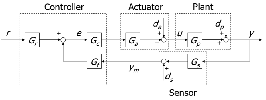
Рис 1: Блок схема системы управления
Думаю, здесь все понятно (di – возмущения).
Постановка задачи:
Найти: Gc(s) и Gf(s) которые удовлетворяют все заданные условия.
Дано: 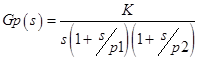 – обьект управления c неопределенностями, которые заданы интервалами:
Для дальнейших расчетов будем использовать номинальные значения, а неопределенности учтем дальше.
Kn=(16+9)/2=12.5,p1n=0.8,p2n=2.5, соответственно получил номинальный объект управления:


Типы возмущений:
Или другими словами это характеристики шума элементов системы.
Рабочие характеристики (performance specifications)
Решение
Очень детально расписывать не буду, только основные моменты.
Одним из ключевых шагов в H∞ методе это определение входных и выходных весовых функций. Эти весовые функции используются для нормирования входа и выхода и отражения временных и частотных зависимостей входных возмущений и рабочих характеристик выходных переменных (ошибок) [1]. Честно говоря, мне это практически ни о чем не говорит, особенно если впервые сталкиваешься с данным методом. В двух словах, весовые функции используются для задания нужный свойств системы управления. Например, в обратной связи стоит сенсор, который имеет шум, обычно высокочастотный, так вот, весовая функция будет своего рода границей, которую контролер не должен пересекать, что бы отфильтровать шум сенсора.
Ниже будем выводить эти весовые функции на основе рабочих характеристик.
- Здесь все просто
- В этом пункте нам нужно определить сколько полюсов в нуле необходимо иметь для контролера (обозначим µ) чтобы удовлетворить Условие 2. Для этого воспользуемся таблицей:
Рис 2: Ошибки по положению, скорости и ускоренияSystem type или астатизм (p) – обозначает количество полюсов в нуле, объекта управления, в нашем случае p=1 (система с астатизмом первого порядка). Так как наш объект управления и есть система с астатизмом 1 порядка, в таком случае полюсов в нуле у контроллера быть не должно. Воспользуемся формулой:
μ+p=h
Где h – порядок входного сигнала, для ramp h=1;
μ=h-p=1-1=0
Теперь воспользуемся теоремой конечных значений, чтобы найти e_r∞
Где e_r – ошибка слежения,
yr – действительный выход (см. Рис 1), уd – желаемый выход
Рис 3: Определение ошибки слеженияВ итоге получим такое:
Это формула установившейся ошибки, неизвестная в данном уравнении S (Sensitivity function)
Где – sensitivity function, L(s) – loop function. Без понятия как они переводятся на русский, оставлю английские названия. Также complementary sensitivity function (как видно из формул, в состав S и T входят Gc – рассчитываемый контроллер, соответственно границы для S и T мы найдем из ошибок и рабочих характеристик, весовые функции определим из S и T, а матлаб из весовых функций найдёт желаемый контроллер.)
В двух словах об S и T [1].
Рис 4: Диаграмма Боде для S,T и LИз графика видно что S ослабляем низкочастотные возмущения, в то время как Т ослабляет высокочастотные возмущения.
- Воспользуемся теоремой конечных значений для e_da
Так как у нас получилось два неравенства найдем условие удовлетворяющее обоих:
Это условие говорит, где Sensitivity function должна пересекать 0 dB axis на диаграмме Боде.
Рис 5: Боде для S - Dp у нас гармоническое возмущение, низкочастотное. Создадим маску для S в районе частот wp
Это значение показывает что S должен находиться ниже -32 dB для частот wp, что бы отфильровать возмущения
Рис 6: Маска для S - Ds также гармоническое возмущение высоких частот, здесь свою роль будет выполнять T
Выполним тоже самое:
Рис 7: Маска для ТКомплексный порядок весовых функций определяется из условии маски и частоты пересечения с 0 осью. В нашем случаи от wp до w примерно одна декада, а так как у нас есть -32 dB то S должен быть минимум 2 порядка. Тоже самое касается и Т.
В итоге схематически ограничение имеют следующий вид для S и Т соответственно:
Рис 8: Все маски для S и T - Для перевода временных характеристик воспользуемся графиками
Рис 9: График зависимости коеффициента демпфирования от переригулированияЗная переригулирование найдем коеффициент демфирования для 10% ->
ξ=0.59
Зная коеффициент демфирования найдем (резонансное) максимально допустимое значение для S и T
Рис 10: График зависимости S_p0 и T_p0 от коеффициента демфированияS_p0=1.35
T_p0=1.05 - Из времени регулирования и настраивания найдем насколько быстрая должна быть система управления
Далее найдем натуральную частоту для S
Натуральная частота для T находим по диаграмме Боде. По условию 5 в частоте 40 rad/s T должен находиться ниже -46 dB, а значит при наклоне в -40 dB/дек натуральная частота должна находиться ниже 4 rad/s. Строя Боде, подбираем оптимальное значение, я получил что:
Рис 11: Боде T-функцииПосле этого у нас есть все данные для построения S T, которые потом трансформируем в весовых функций. S T имеют следующую форму:
Обычно для построения весовых функций используют Butterworth коэффициенты
Весовые функции имеют вид:
Для все просто, и нас есть все необходимое, что бы подставить в формулу. Для нужно еще несколько расчетов.
Так как рабочие характеристики дают нам граничные условия в рамках которых наш контроллер будет выполнять все условия. Весовые функции объединяют в себе все условия и потом используются как правая и левая граница в которых находиться контроллер удовлетворяющий все условия.
Для
 Здесь все просто
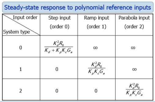
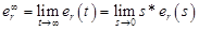
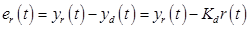
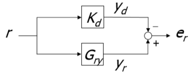
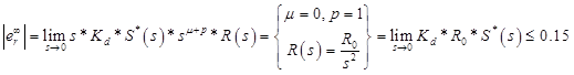

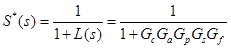 – sensitivity function, L(s) – loop function. Без понятия как они переводятся на русский, оставлю английские названия. Также complementary sensitivity function
  (как видно из формул, в состав S и T входят Gc – рассчитываемый контроллер, соответственно границы для S и T мы найдем из ошибок и рабочих характеристик, весовые функции определим из S и T, а матлаб из весовых функций найдёт желаемый контроллер.)
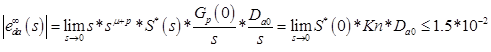


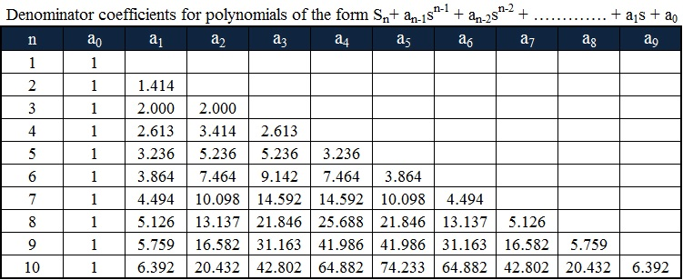

 все просто, и нас есть все необходимое, что бы подставить в формулу. Для
  нужно еще несколько расчетов.
В итоге получим:
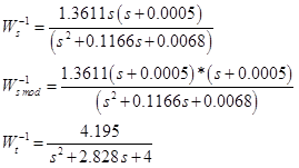
Generalized plant
Hinf метод или метод минимизации бесконечной нормы Hinfinity относится к общей формулировке проблемы управления которая основывается на следующей схеме представления системы управления с обратной связью:

Рис 12: Обобщенный схема системы управления
Перейдем к пункту расчета контроллера и что для этого нужно. Изучение алгоритмов расчета нам не объясняли, говорили: «делайте вот так и все получиться», но принцип вполне логичен. Контроллер получается в ходе решения оптимизационной задачи:
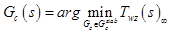
 – замкнутая передаточная функция от W к Z.
Сейчас нам нужно составить generalized plant (пунктирный прямоугольник рис ниже). Gpn мы уже определили, это номинальный объект управления. Gc — контроллер который мы получим в итоге. W1 = Ws(s), W2 = max (WT(s),Wu(s)) – это весовые функции определенные ранее. Wu(s) – это весовая функция неопределенности, давайте ее определим.
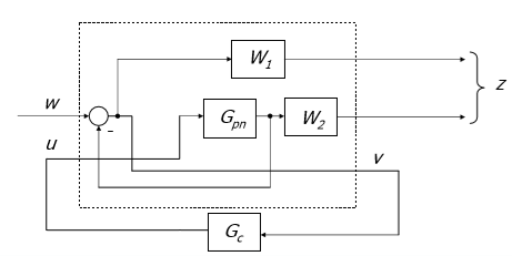
Рис 13: Раскрытая схемы управления
Wu(s)
Предположим что имеем мультипликативные неопределенности в объекте управления, можно изобразить так:

Рис 14: Мультипликативная неопределенность
И так для нахождения Wu воспользуемся матлаб. Нам нужно построить Bode все возможных отклонений от номинального объекта управления, и потом построить передаточную функцию которая опишет все эти неопределенности:
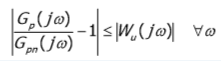
Сделаем примерно по 4 прохода для каждого параметра и построим bode. В итоге получим такое:

Рис 15: Диграмма Боде неопределенностей
Wu будет лежать выше этих линий. В матлаб есть tool который позволяем мышкой указать точки и по этим точкам строит передаточную функцию.
Kод
mf = ginput(20);
magg = vpck(mf(:,2),mf(:,1));
Wa = fitmag(magg);
[A,B,C,D]=unpck(Wa);
[Z,P,K]=ss2zp(A,B,C,D);
Wu = zpk(Z,P,K)
После введения точек старится кривая и предлагается ввести степень передаточной функции, введем степень 2.
Вот что получилось:
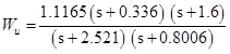
Теперь определим W2, для этого построим Wt и Wu:
Из графика видно что Wt больше Wu значит W2 = Wt.

Рис 16: Опредиление W2
Дальше нам нужно в симулинке построить generalized plant как сделано ниже:
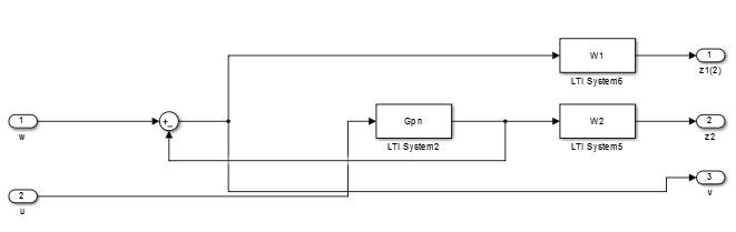
Рис 17: Блок схема Generalized plant в simulink
И сохранить под именем, например g_plant.mdl
Один важный момент:
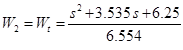 — not proper tf, если мы ее оставим так то нам выдаст ошибку. По этому заменяем на
  и потом добавим два нуля к выходу z2 с помощью “sderiv“.
Реализация в матаб
p = 2; % частота нулей в районе частоты Т функции
[Am,Bm,Cm,Dm] = linmod(‘g_plant’);
M = ltisys(Am,Bm,Cm,Dm);
M = sderiv(M,2,[1/p 1]);
M = sderiv(M,2,[1/p 1]);
[gopt,Gcmod] = hinflmi(M,[1 1],0,0.01,[0,0,0]);
[Ac,Bc,Cc,Dc] = ltiss(Gcmod);
[Gc_z,Gc_p,Gc_k] = ss2zp(Ac,Bc,Cc,Dc);
Gc_op = zpk(Gc_z,Gc_p,Gc_k)
После выполнения этого кода получаем контроллер:
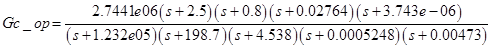
В принципе можно так и оставить, но обычно удаляют низко- и высокочастотные нули и полюсы. Таким образом мы уменьшаем порядок контроллера. И получаем следующий контроллер:
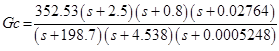
получим вот такой Hichols chart:
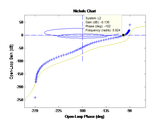
Рис 18: Hichols chart разомкнутой системы с полученным контроллером
И Step response:

Рис 19: Переходная характеристика замкнутой системы с контроллером
А теперь самое сладкое. Получился ли наш контроллер робастным или нет. Для этого эксперимента просто нужно изменить наш объект управления (коэффициенты к, р1, р2) и посмотреть step response и интересующими характеристиками, в нашем случае это перерегулирование, время регулирования для 5 % и время нарастания [2].

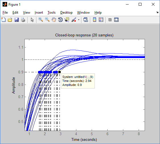
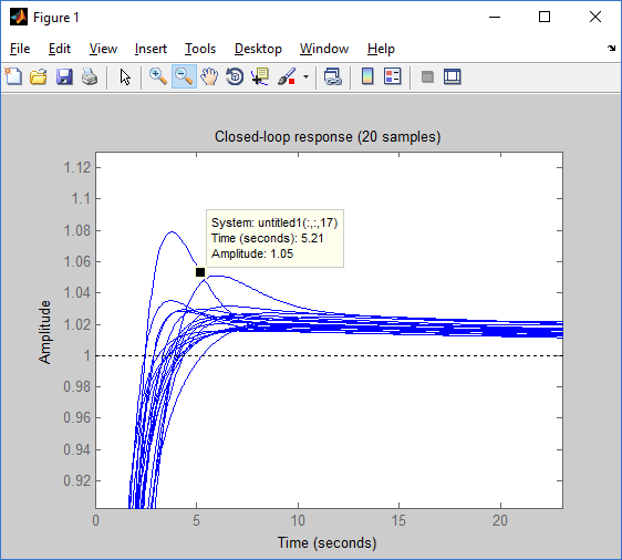
Рис 20: Временные характеристики для разных параметров объект управления
Построив 20 разных переходных характеристик, я выделил максимальные значения для каждой временной характеристики:
• Максимальное переригулирование – 7.89 %
• Макс время нарастания – 2.94 сек
• Макс время регелирования 5% — 5.21 сек
И о чудо, характеристики там где нужно не только для номинального обьекта, но и для интервала параметров.
А сейчас сравним с классичиским ПИД контролером, и посмотрим стоила игра свеч или нет.
ПИД расчитал pidtool для номинального обьекта управления (см выше):
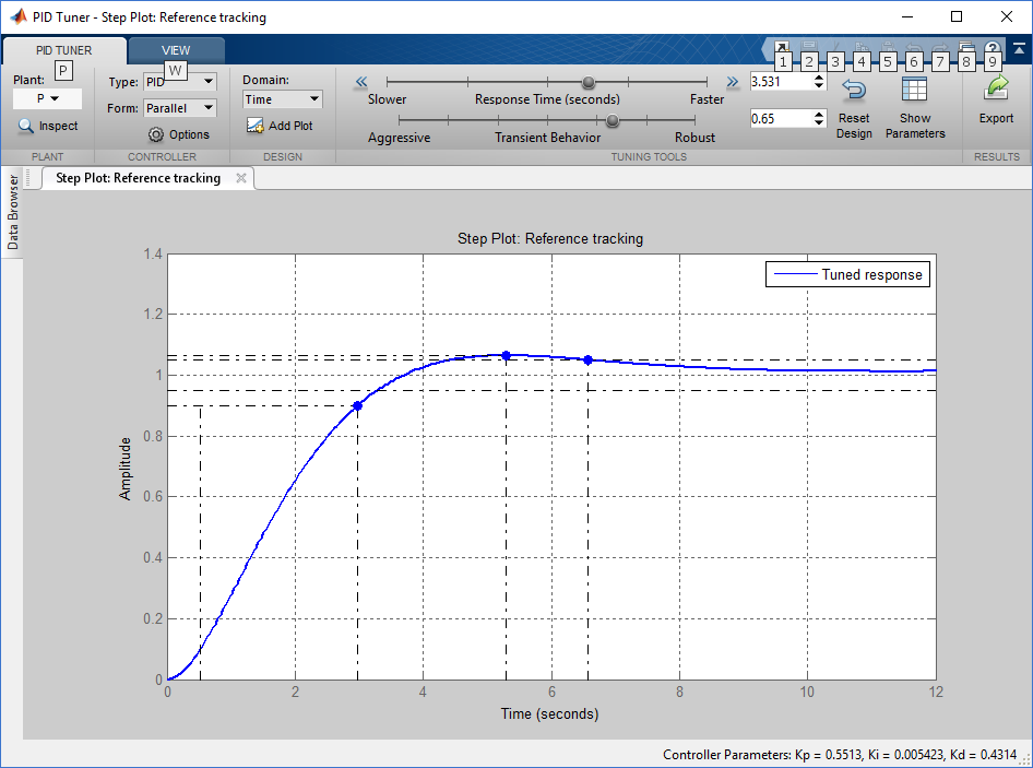
Рис 21: Pidtool
Получим такой контроллер:
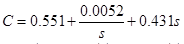
Теперь H-infinity vs PID:

Рис 22: H-infinity vs PID
Видно что ПИД не справляется с такими неопределенностями и ПХ выходит за заданные ограничения, в то время как робастные контроллер «жестко» держат систему в заданных интервалах перерегулирования, времени нарастания и регулирования.
Что бы не удлинять статью и не утомлять читателя, опущу проверку характеристики 2-5 (ошибки), скажу, что в случае робастного контроллера все ошибки находятся ниже заданных, также был проведен тест с другими параметрами объекта:

Ошибки находились ниже заданных, что означает, что данный контроллер полностью справляется с поставленной задачей. В то время как ПИД не справился только с пунктом 4 (ошибка dp).
На этом все по расчету контроллера. Критикуйте, спрашивайте.
Ссылка на файл матлаб: drive.google.com/open?id=0B2bwDQSqccAZTWFhN3kxcy1SY0E
Список литературы
1. Guidelines for the Selection of Weighting Functions for H-Infinity Control
2. it.mathworks.com/help/robust/examples/robustness-of-servo-controller-for-dc-motor.html
РОБАСТНЫЙ АНАЛИЗ
C.1 Введение
Межлабораторные сравнительные испытания представляют собой особый анализ данных. В то время как большинство межлабораторных сравнительных испытаний представляют данные, подчиняющиеся унимодальному и приблизительно симметричному распределению в задачах проверки квалификации, большая часть наборов данных включает часть результатов, неожиданно далеко отстоящих от основного набора данных. Причины появления таких данных могут быть различными: например, появление новых, менее опытных участников проверки, появление новых и, возможно, менее точных методов измерений, непонимание некоторыми участниками инструкции или неправильная обработка образцов. Такие отличающиеся результаты (выбросы) могут быть весьма изменчивы, в этом случае применение традиционных статистических методов, в том числе вычисление среднего арифметического и стандартного отклонений, может дать недостоверные результаты.
Провайдерам рекомендуется (см. 6.5.1) использовать статистические методы, устойчивые к выбросам. Большинство таких методов предложено в книгах по математической статистике, и многие из них успешно использованы в задачах проверки квалификации. Обычно робастные методы обеспечивают дополнительную устойчивость при обработке данных из асимметричных распределений с выбросами.
В данном приложении описано несколько простых в применении методов, используемых в задачах проверки квалификации и имеющих различные возможности в отношении определения устойчивости оценок при наличии данных из загрязненных совокупностей (например, эффективности и пороговой точки). Методы представлены в порядке возрастания сложности (первый — самый простой, последний — самый сложный), и в порядке убывания эффективности, поэтому наиболее сложные оценки требуют доработки для повышения их эффективности.
Примечание 1 — В приложении D приведена дополнительная информация об эффективности, пороговых точках и чувствительности к небольшим модам — трем важным показателям различных робастных методов определения оценки функционирования.
Примечание 2 — Робастность является свойством алгоритма определения оценки, а не свойством полученных оценок, поэтому не совсем корректно называть средние значения и стандартные отклонения, рассчитанные с помощью такого алгоритма, робастными. Однако, чтобы избежать использования чрезмерно громоздких терминов, в настоящем стандарте применены термины «робастное среднее» и «робастное стандартное отклонение». Следует учитывать, что это означает оценки среднего или стандартного отклонения, полученные в соответствии с робастным алгоритмом.
C.2 Простые устойчивые к выбросам оценки для среднего и стандартного отклонений совокупности
C.2.1 Медиана
Медиана является наиболее простой, высоко устойчивой к выбросам оценкой среднего для симметричного распределения. Обозначим медиану med(x). Для определения med(x) по совокупности из p данных необходимо:
i) расположить p данных в порядке неубывания:
x{1}, x{2}, …, x{p};
ii) вычислить
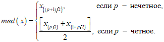 (C.1)
(C.1)
C.2.2 Абсолютное отклонение от медианы MADe
Абсолютное отклонение от медианы MADe(x) обеспечивает определение оценки стандартного отклонения генеральной совокупности для данных из нормального распределения и является высоко устойчивым при наличии выбросов. Для определения MADe(x) вычисляют:
i) абсолютные значения разностей di(i = 1, …, p)
di = |xi — med(x)|; (C.2)
ii) MADe(x)
MADe(x) = 1,483 med(d). (C.3)
Если у половины или большего количества участников результаты совпадают, то MADe(x) = 0, и следует использовать оценку n/QR в соответствии с C.2.3, стандартное отклонение, полученное после исключения выбросов, или процедуру, описанную в C.5.2.
C.2.3 Нормированный межквартильный размах n/QR
Данный метод определения робастной оценки стандартного отклонения аналогичен методу определения MADe(x). Эту оценку получить немного проще, поэтому ее часто используют в программах проверки квалификации. Данную оценку определяют как разность 75-го процентиля (или 3-го квартиля) и 25-го процентиля (или 1-го квартиля) результатов участника. Данную статистику называют нормированным межквартильным размахом n/QR и вычисляют по формуле
n/QR(x) = 0,7413(Q3(x) — Q1(x)), (C.4)
где Q1(x) — 25-й процентиль выборки xi(i = 1, 2, …, p);
Q3(x) — 75-й процентиль выборки xi(i = 1, 2, …, p).
Если 75-й и 25-й процентили совпадают, то n/QR = 0 [как и MADe(x)], а для вычисления робастного стандартного отклонения следует использовать альтернативную процедуру, такую как арифметическое стандартное отклонение (после исключения выбросов), или процедуру, описанную в C.5.2.
Примечание 1 — Для расчета n/QR требуется сортировка данных только один раз в отличие от вычисления MADe, но n/QR имеет пороговую точку в 25% (см. приложение D), в то время как у MADe пороговая точка 50%. Поэтому MADe устойчива при значительно более высокой доле содержания выбросов, чем n/QR.
Примечание 2 — При p < 30 обе оценки обладают заметным отрицательным смещением, неблагоприятно влияющим на оценки участников при проверке квалификации.
Примечание 3 — Различные пакеты статистических программ используют различные алгоритмы расчета квартилей и, следовательно, могут давать оценки n/QR с некоторыми различиями.
Примечание 4 — Пример использования робастных оценок приведен в E.3 приложения E.
C.3 Алгоритм A
C.3.1 Алгоритм A с итеративной шкалой
Данный алгоритм дает робастные оценки среднего и стандартного отклонения на основе используемых данных.
Для выполнения алгоритма A p данные располагают в порядке неубывания
x{1}, x{2}, …, x{p}.
Полученные по этим данным робастное среднее и робастное стандартное отклонения обозначают x* и s*.
Вычисляют начальные значения для x* и s* по формулам:
x* = med(xi)(i = 1, 2, …, p), (C.5)
s* = 1,483 med|xi — x*|, (i = 1, 2, …, p). (C.6)
Примечание 1 — Алгоритмы A и S, приведенные в настоящем приложении, соответствуют ГОСТ Р ИСО 5725-5 с добавлением критерия остановки: при совпадении до 3-го знака после запятой среднего и стандартного отклонения вычисления прекращают.
Примечание 2 — В некоторых случаях более половины результатов xi будут идентичны (например, количество нитей в образцах ткани или количество электролитов в образцах сыворотки крови). В этом случае начальное значение s* = 0 и робастная процедура будут некорректными. Если начальное значение s* = 0, допустимо заменить выборочное стандартное отклонение после проверки всех очевидных выбросов, которые могут сделать стандартное отклонение неоправданно большим. Такую замену проводят только для начального значения s* и после этого итеративный алгоритм применяют в соответствии с описанием.
Вычисляют новые значения x* и s*. Для этого вычисляют
 . (C.7)
Для каждого xi(i = 1, 2, …, p) вычисляют
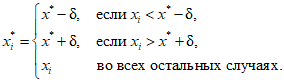 (C.8)
(C.8)
Вычисляют новые значения x* и s*
 , (C.9)
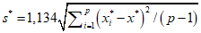 , (C.10)
где суммирование производят по i.
Робастные оценки x* и s* получают на основе итеративных, то есть повторных вычислений x* и s* в соответствии с (C.7) — (C.10) до тех пор, пока процесс не начнет сходиться, то есть разности предыдущих и последующих значений x* и s* не станут пренебрежимо малы. Обычно итеративные вычисления прекращают при совпадении в предыдущих и последующих значениях трех знаков после запятой.
Альтернативные критерии сходимости могут быть определены в соответствии с требованиями к плану эксперимента и к отчету по результатам проверки квалификации.
Примечание — Примеры использования алгоритма A приведены в E.3 и E.4 приложения E.
C.3.2 Варианты алгоритма A
Итеративный алгоритм A, приведенный в C.3.1, имеет скромную разбивку (примерно 25% для больших наборов данных [14]) и начальную точку для s*, предложенную в C.3.1, для наборов данных, где MADe(x) = 0 может серьезно ухудшить устойчивость при наличии нескольких выбросов в наборе данных. Если в наборе данных ожидаемая доля выбросов составляет более 20% или если начальное значение s* подвержено неблагоприятному влиянию экстремальных выбросов, то следует рассмотреть следующие варианты:
i) замена MADe на  при MADe = 0 либо использование альтернативной оценки в соответствии с C.5.1 или арифметического стандартного отклонения (после исключения выбросов);
ii) если при оценке робастное стандартное отклонение не используют, следует применять MADe [исправленное в соответствии с i)], и не изменяют s* во время итерации. Если при оценке используют робастное стандартное отклонение, заменяют s* в соответствии с C.5 оценкой Q и не изменяют s* во время итерации.
Примечание — Вариант, приведенный в перечислении ii), улучшает пороговую точку алгоритма A до 50% [14], что позволяет применять алгоритм при наличии высокой доли выбросов.
C.4 Алгоритм S
Данный алгоритм применяют к стандартным отклонениям (или размахам), которые вычисляют, если участники представляют результаты m репликаций измерений измеряемой величины образца или в исследовании используют m идентичных образцов. Алгоритм позволяет получить робастное объединенное значение стандартных отклонений или размахов.
Имеющиеся p стандартных отклонений или размахов располагают в порядке неубывания
w{1}, w{2}, …, w{p}.
Обозначим робастное объединенное значение w*, а v — число степеней свободы, соответствующее каждому wi. (Если wi — размах, то v = 1. Если wi — стандартное отклонение для m результатов испытаний, то v = m — 1.) Значения ![]() и
и ![]() определяют в соответствии с алгоритмом, приведенным в таблице C.1.
определяют в соответствии с алгоритмом, приведенным в таблице C.1.
Вычисляют начальное значение w*:
w* = med(wi), (i = 1, 2, …, p). (C.11)
Примечание — Если более половины wi имеют значения, равные нулю, то начальное значение w* равно нулю, а робастный метод является некорректным. Если начальное значение w* равно нулю, то после устранения выбросов, которые могут повлиять на выборочное среднее, заменяют стандартное отклонение объединенного среднего арифметического (или размах средних арифметических). Эту замену выполняют только для начального значения w*, после чего процедуру продолжают согласно описанию.
Значение w* вычисляют следующим образом:
 . (C.12)
Для каждого значения wi(i = 1, 2, …, p) вычисляют
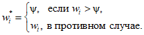 (C.13)
Вычисляют новое значение w*
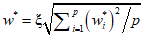 . (C.14)
Робастную оценку w* получают итеративным методом, вычисляя значение w* несколько раз, пока процесс не начнет сходиться. Сходимость считают достигнутой, если значения w* в последовательных итерациях совпадают в трех знаках после запятой.
Примечание — Алгоритм S обеспечивает оценку стандартного отклонения генеральной совокупности, если оно получено по стандартным отклонениям из того же нормального распределения (и, следовательно, обеспечивает оценку стандартного отклонения повторяемости при выполнении предположений в соответствии с ГОСТ Р ИСО 5725-2).
Таблица C.1
Коэффициенты, необходимые для проведения
робастного анализа: алгоритм S
|
Число степеней свободы v |
Лимитирующий коэффициент |
Поправочный коэффициент |
|
1 |
1,645 |
1,097 |
|
2 |
1,517 |
1,054 |
|
3 |
1,444 |
1,039 |
|
4 |
1,395 |
1,032 |
|
5 |
1,359 |
1,027 |
|
6 |
1,332 |
1,024 |
|
7 |
1,310 |
1,021 |
|
8 |
1,292 |
1,019 |
|
9 |
1,277 |
1,018 |
|
10 |
1,264 |
1,017 |
|
Примечание — Значения |
C.5 Сложные для вычислений робастные оценки: Q-метод и оценка Хампеля
C.5.1 Обоснование оценок
Робастные оценки среднего и стандартного отклонения генеральной совокупности, описанные в C.2 и C.3, используют в тех случаях, когда вычислительные ресурсы ограничены или когда требуется краткое обоснование статистических процедур. Эти процедуры оказались полезными в самых разных ситуациях, в том числе в программах проверки квалификации в новых областях исследований или при калибровке и в тех областях экономики, где проверка квалификации раньше не была доступна. Однако эти методы являются недостоверными в тех случаях, когда количество выбросов в результатах превышает 20%, или в случае бимодального (или мультимодального) распределения данных, и некоторые из них могут стать неприемлемо изменчивыми для небольшого количества участников. Кроме того, ни один из этих методов не может работать с данными репликаций измерений участников. В соответствии с ГОСТ ISO/IEC 17043 необходимо, чтобы эти ситуации были предусмотрены до проведения расчетов или выполнены в процессе анализа до проведения оценки функционирования участника, однако это не всегда возможно.
Кроме того, некоторые робастные методы, описанные в C.2 и C.3, имеют низкую статистическую эффективность. Если количество участников менее 50, а робастное среднее и/или стандартное отклонение используют для определения индексов, то существует значимый риск неверной классификации участников при применении неэффективных статистических методов.
Робастные методы, объединяющие высокую эффективность (то есть сравнительно низкую изменчивость) с возможностью работы с высокой долей выбросов в данных, обычно являются достаточно сложными и требуют серьезных вычислительных ресурсов, но эти методы представлены в литературе и международных стандартах. Некоторые из них обеспечивают получение дополнительных преимуществ, когда основное распределение данных является асимметричным или определенные результаты находятся ниже предела их обнаружения.
Ниже приведены некоторые высокоэффективные методы определения оценок стандартного отклонения и параметра положения (среднего), которые показывают более низкую изменчивость, чем простые оценки, и полезны при использовании для данных с большой долей выбросов. Одну из описанных оценок можно применять для оценки стандартного отклонения воспроизводимости, если участники сообщают о большом количестве наблюдений.
C.5.2 Определение робастного стандартного отклонения с использованием Q-метода и Qn-метода
C.5.2.1 Оценка Qn [15] является высокоэффективной оценкой стандартного отклонения генеральной совокупности с разбивкой, которая становится несмещенной для данных нормального распределения (при условии отсутствия выбросов).
Qn-метод учитывает единственный результат для каждого участника (включающий среднее или медиану репликаций измерений). Расчет основан на использовании попарных различий в наборе данных и поэтому не зависит от оценки среднего или медианы.
Выполнение этого метода включает корректировки, позволяющие обеспечить несмещенность оценки для всех фактических объемов наборов данных.
При вычислении Qn для набора данных (x1, x2, …, xp) с p результатами:
i) вычисляют p(p — 1)/2 абсолютных разностей
dij = |xi — xj| для i = 1, 2, …, p,
j = i + 1, i + 2, …, p; (C.15)
ii) для разностей dij используют обозначения
d{1}, d{2}, …, d{p(p-1)/2; (C.16)
iii) вычисляют
 , (C.17)
где k — количество различных пар, выбранных из h объектов,
где
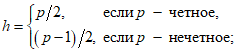 (C.18)
iv) вычисляют Qn
Qn = 2,2219d(k)bp, (C.19)
где bp определяют по таблице C.2 для конкретного количества данных, если p > 12, bp вычисляют по формуле
 , (C.20)
где
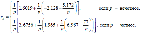 (C.21)
Примечание 1 — Коэффициент 2,2219 является поправочным, обеспечивающим несмещенность оценки стандартного отклонения для больших p. Поправочные коэффициенты bp для небольших значений p определяют по таблице C.2, а при p > 12 эти коэффициенты устанавливают в соответствии с [15], используя экстенсивное моделирование и последующее применение регрессионного анализа.
Примечание 2 — Простой алгоритм, описанный выше, для больших наборов данных, например, при p > 1000, требует значительных вычислительных ресурсов. Для быстрой обработки опубликованы программы (см. [15]) для использования с более крупными наборами данных (на момент публикации приведена обработка данных с объемом выше 8000 за приемлемое время).
Таблица C.2
Поправочный коэффициент bp для 2 <= p <= 12
|
p |
2 |
3 |
4 |
5 |
6 |
7 |
8 |
9 |
10 |
11 |
12 |
|
bp |
0,9937 |
0,9937 |
0,5132 |
0,8440 |
0,6122 |
0,8588 |
0,6699 |
0,8734 |
0,7201 |
0,8891 |
0,7574 |
C.5.2.2 Q-метод позволяет получить высокоэффективную оценку стандартного отклонения результатов проверки квалификации, представленных различными лабораториями, с разбивкой. Q-метод не является устойчивым не только при наличии выбросов, но и в той ситуации, когда большая часть результатов испытаний равны между собой, например, когда результаты представляют собой дискретные числа или при округлении данных. В такой ситуации другие подобные методы не следует применять, поскольку многие разности равны нулю.
Q-метод можно использовать для проверки квалификации как в случае предоставления участником единственного результата (в виде среднего и медианы репликаций измерений), так и результатов репликаций. Прямое использование репликаций измерений в вычислениях повышает эффективность метода.
Расчет основан на использовании разностей пар в наборе данных, и таким образом оценка не зависит от оценки среднего или медианы данных. Метод называют Q-методом, или методом Хампеля, если его используют вместе с алгоритмом конечных шагов для определения оценки Хампеля, описанной в C.5.3.3.
Обозначим результаты измерений участников, сгруппированные по лабораториям
 .
.
Кумулятивная функция распределения абсолютных значений разностей результатов участников имеет следующий вид:
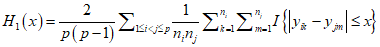 , (C.22)
где 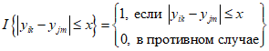 — индикаторная функция.
Обозначим точки разрыва функции H1(x):
x1, …, xr, где x1 < x2 < … < xr.
Значения функции в точках x1, …, xr
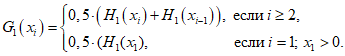 (C.23)
Пусть G1(0) = 0.
Значения функции G1(x) для x вне интервала [0, xr] вычисляют с помощью линейной интерполяции между точками разрыва 0 <= x1 < x2 < … < xr.
Робастное стандартное отклонение s* результатов испытаний для различных лабораторий имеет вид:
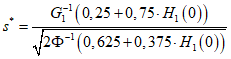 , (C.24)
где H1(0) вычисляют аналогично формуле (C.22) и H1(0) = 0 в случае точного совпадения данных, и ![]() — квантиль стандартного нормального распределения уровня q.
— квантиль стандартного нормального распределения уровня q.
Примечание 1 — Этот алгоритм не зависит от среднего, он может быть использован либо вместе со значением, полученным по объединенным результатам участников, или в соответствии с установленным опорным значением.
Примечание 2 — Другие варианты Q-метода, позволяющие получить робастную оценку стандартных отклонений воспроизводимости и повторяемости, приведены в [14], [15].
Примечание 3 — Теоретические основы Q-метода, включая его асимптотическую эффективность и разбивку на конечное число выборок, описаны в [16] и [15].
Примечание 4 — Если исходные данные участников представлены единственным результатом измерений, полученным с помощью одного установленного метода измерений, робастное стандартное отклонение является оценкой стандартного отклонения воспроизводимости, как и в (C.21).
Примечание 5 — Стандартное отклонение воспроизводимости не обязательно является наиболее подходящим стандартным отклонением для использования в проверке квалификации, так как это, как правило, оценка разброса единственных результатов, а не оценка разброса средних или медиан результатов репликаций каждого участника. Однако разброс средних или медиан результатов репликаций лишь немного менее разброса единственных результатов различных лабораторий, если отношение стандартного отклонения воспроизводимости к стандартному отклонению повторяемости более двух. Если это отношение менее двух, для определения оценок при проверке квалификации может быть использована замена стандартного отклонения воспроизводимости sR скорректированным значением
 ,
,
где m — количество репликаций;
![]() — дисперсия повторяемости, вычисленная в соответствии с [17], или можно использовать среднее значение репликаций измерений участника Q-метода.
— дисперсия повторяемости, вычисленная в соответствии с [17], или можно использовать среднее значение репликаций измерений участника Q-метода.
Примечание 6 — Примечание 5 применяют только в том случае, если индексы определяют на основе средних или медиан результатов репликаций. Если репликации проводят вслепую, индексы следует рассчитывать для каждой репликации. В этом случае стандартное отклонение воспроизводимости является наиболее подходящим стандартным отклонением.
Примечание 7 — Пример применения Q-метода приведен в E.3 приложения E.
C.5.3 Определение робастного среднего, используемого в оценке Хампеля
C.5.3.1 Оценка Хампеля является высокоустойчивой высокоэффективной оценкой общего среднего всех результатов различных лабораторий. Поскольку формулы вычисления оценки Хампеля не существует, ниже приведены два алгоритма получения этой оценки. Первый из них является более простым, но может привести к отклонениям результатов при выполнении. Второй алгоритм обеспечивает получение однозначных результатов, зависящих только от базового стандартного отклонения.
C.5.3.2 Далее приведены вычисления, обеспечивающие получение итеративной взвешенной оценки Хампеля, для параметра положения.
i) Пусть x1, x2, …, xp — данные.
ii) Пусть x* — медиана med(x) (см. C.2.1).
iii) Пусть s* — соответствующая робастная оценка стандартного отклонения, например, MADe, Qn или s* в соответствии с Q-методом.
iv) Для каждой точки xi вычисляют qi
 .
.
v) Вычисляют вес wi
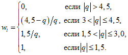
vi) Пересчитывают x*
 .
.
vii) Повторяют действия в соответствии с перечислениями iv) — vi) до тех пор, пока значения x* не начнут сходиться. Сходимость считают достаточной, если разность x* в двух последних итерациях станет менее  , что соответствует приблизительно 1% стандартной погрешности x*. Могут быть использованы и другие более точные критерии сходимости.
Данный алгоритм получения оценки Хампеля не гарантирует получение единственной и наилучшей оценки, так как неудачный выбор начального значения x* и/или s* может привести к исключению важной части набора данных. Провайдеру следует предпринять соответствующие меры для проверки возможности получения неудачного результата или обеспечить однозначные правила выбора параметра положения. Наиболее общим правилом является выбор параметра положения, максимально близкого к медиане. Анализ результатов для подтверждения того, что большая часть данных не выходит за пределы области |q| > 4,5, может также помочь в принятии правильного решения.
Примечание 1 — Определение оценки Хампеля для данных из нормального распределения обладает эффективностью, приблизительно равной 96%.
Примечание 2 — Примеры выполнения этого алгоритма приведены в E.3 приложения E.
Примечание 3 — Эффективность и устойчивость к выбросам оценки Хампеля могут быть повышены с помощью изменения весовой функции. Общая форма весовой функции имеет вид:
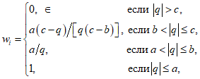
где a, b и c — регулируемые параметры. Для приведенного алгоритма a = 1,5, b = 3,0 и c = 4,5. Более высокая эффективность достигается за счет увеличения области изменений q. Повышения устойчивости к выбросам или изменениям режимов достигают за счет уменьшения области изменений q.
C.5.3.3 Ниже приведен алгоритм конечных шагов, позволяющий получить оценку Хампеля для параметра положения [14].
Вычисляют средние арифметические y1, y2, …, yp.
Вычисляют робастное среднее x* как корень уравнения
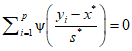 , (C.25)
где
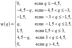 (C.26)
s* — робастное стандартное отклонение, полученное Q-методом.
Точное решение может быть получено за конечное число шагов, без итерации, используя свойство, при котором ![]() как функция x* является частично линейной, имея в виду точки интерполяции в левой стороне уравнения (C.25).
как функция x* является частично линейной, имея в виду точки интерполяции в левой стороне уравнения (C.25).
Вычисляют все точки интерполяции:
— для 1-го значения y1:
d1 = y1 — 4,5·s*, d2 = y1 — 3·s*, d3 = y1 — 1,5·s*,
d4 = y1 + 1,5·s*, d5 = y1 + 3·s*, d6 = y1 + 4,5s*;
— для 2-го значения y2:
d7 = y2 — 4,5·s*, d8 = y2 — 3·s*, d9 = y2 — 1,5·s*,
d10 = y2 + 1,5·s*, d11 = y2 + 3·s*, d12 = y2 + 4,5·s*;
— и так далее для всех y3, …, yp.
Располагают d1, d2, d3, …, d6·p в порядке неубывания d{1}, d{2}, d{3}, …, d{6·p}.
Затем для каждого m = 1, …, (6·p — 1) вычисляют
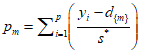
и проверяют, являются ли следующие условия:
(i) если pm = 0, то d{m} — решение уравнения (C.25);
(ii) если pm+1 = 0, то, d{m+1} — решение уравнения (C.25);
(iii) если pm·pm+1 < 0, то 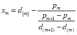 — решение уравнения (C.25).
Пусть S — множество всех решений уравнения (C.25).
Решением ![]() является ближайшая медиана, используемая в качестве параметра положения x*, то есть
является ближайшая медиана, используемая в качестве параметра положения x*, то есть
 .
.
Могут существовать несколько решений. Если существуют два решения, наиболее близких к медиане, или если не существует никакого решения вообще, то в качестве параметра положения x* используют медиану.
Примечание 1 — Эта оценка Хампеля для данных из нормального распределения обладает эффективностью, приблизительно равной 96%.
Примечание 2 — При использовании этого метода результаты лабораторий, отличающиеся от среднего более чем на 4,5 стандартных отклонений воспроизводимости, не оказывают никакого влияния на результат, то есть их рассматривают как выбросы.
C.5.4 Метод Q/Хампеля
Метод Q/Хампеля использует Q-метод, описанный в C.5.3.2, для вычисления робастного стандартного отклонения s* и алгоритм конечных шагов для оценки Хампеля, описанный в C.5.3.3, для вычисления параметра положения x*.
Если участники сообщают много наблюдений для вычисления робастного стандартного отклонения воспроизводимости sR, используют Q-метод, описанный в C.5.3.2. Для вычисления робастного стандартного отклонения повторяемости sr применяют 2-й алгоритм, использующий парные разности в пределах лаборатории.
Примечание — Веб-приложения для метода Q/Хампеля приведены в [18].
C.6 Другие робастные методы
Методы, описанные в настоящем приложении, не представляют собой целостную совокупность всех подходов. Ни один из них не является гарантированно оптимальным во всех ситуациях. По усмотрению провайдера могут быть использованы другие робастные методы при условии анализа их эффективности и всех остальных свойств, соответствующих определенным требованиям программы проверки квалификации.
Приложение D
(справочное)
Скачать документ целиком в формате PDF
Так как гетероскедастичность не приводит к смещению оценок коэффициентов, можно по-прежнему использовать МНК. Смещены и несостоятельны оказываются не сами оценки коэффициентов, а их стандартные ошибки, поэтому формула для расчета стандартных ошибок в условиях гомоскедастичности не подходит для случая гетероскедастичности.
Естественной идеей в этой ситуации является корректировка формулы расчета стандартных ошибок, чтобы она давала «правильный» (состоятельный) результат. Тогда можно снова будет корректно проводить тесты, проверяющие, например, незначимость коэффициентов, и строить доверительные интервалы. Соответствующие «правильные» стандартные ошибки называются состоятельными в условиях гетероскедастичности стандартными ошибками (heteroskedasticity consistent (heteroskedasticity robust) standard errors)1. Первоначальная формула для их расчета была предложена Уайтом, поэтому иногда их также называют стандартными ошибками в форме Уайта (White standard errors). Предложенная Уайтом состоятельная оценка ковариационной матрицы вектора оценок коэффициентов имеет вид:
(widehat{V}{left( widehat{beta} right) = n}left( {X^{‘}X} right)^{- 1}left( {frac{1}{n}{sumlimits_{s = 1}^{n}e_{s}^{2}}x_{s}x_{s}^{‘}} right)left( {X^{‘}X} right)^{- 1},)
где (x_{s}) – это s-я строка матрицы регрессоров X. Легко видеть, что эта формула более громоздка, чем формула (widehat{V}{left( widehat{beta} right) = left( {X^{‘}X} right)^{- 1}}S^{2}), которую мы вывели в третьей главе для случая гомоскедастичности. К счастью, на практике соответствующие вычисления не представляют сложности, так как возможность автоматически рассчитывать стандартные ошибки в форме Уайта реализована во всех современных эконометрических пакетах. Общепринятое обозначение для этой версии стандартных ошибок: «HC0». В работах (MacKinnon, White,1985) и (Davidson, MacKinnon, 2004) были предложены и альтернативные версии, которые обычно обозначаются в эконометрических пакетах «HC1», «HC2» и «HC3». Их расчетные формулы несколько отличаются, однако суть остается прежней: они позволяют состоятельно оценивать стандартные отклонения МНК-оценок коэффициентов в условиях гетероскедастичности.
Для случая парной регрессии состоятельная в условиях гетероскедастичности стандартная ошибка оценки коэффициента при регрессоре имеет вид:
(mathit{se}{left( widehat{beta_{2}} right) = sqrt{frac{1}{n}frac{frac{1}{n — 2}{sumlimits_{i = 1}^{n}{left( {x_{i} — overline{x}} right)^{2}e_{i}^{2}}}}{widehat{mathit{var}}(x)^{2}}.}})
Формальное доказательство состоятельности будет приведено в следующей главе. Пока же обсудим пример, иллюстрирующий важность использования робастных стандартных ошибок.
Пример 5.1. Оценка эффективности использования удобрений
В файле Agriculture в материалах к этому учебнику содержатся следующие данные 2010 года об урожайности яровой и озимой пшеницы в Спасском районе Пензенской области:
PRODP — урожайность в денежном выражении, в тысячах рублей с 1 га,
SIZE – размер пахотного поля, га,
LABOUR – трудозатраты, руб. на 1 га,
FUNG1 – фунгициды, протравители семян, расходы на удобрение в руб. на 1 га,
FUNG2 – фунгициды, во время роста, расходы на удобрение в руб. на 1 га,
GIRB – гербициды, расходы на удобрение в руб. на 1 га,
INSEC – инсектициды, расходы на удобрение в руб. на 1 га,
YDOB1 – аммофос, во время сева, расходы на удобрение в руб. на 1 га,
YDOB2 – аммиачная селитра, во время роста, расходы на удобрение в руб. на 1 га.
Представим, что вас интересует ответ на вопрос: влияет ли использование фунгицидов на урожайность поля?
(а) Оцените зависимость урожайности в денежном выражении от константы и переменных FUNG1, FUNG2, YDOB1, YDOB2, GIRB, INSEC, LABOUR. Запишите уравнение регрессии в стандартной форме, указав коэффициент детерминации и (в скобках под соответствующими коэффициентами) стандартные ошибки для случая гомоскедастичности. Какие из переменных значимы на 5-процентном уровне значимости?
(б) Решите предыдущий пункт заново, используя теперь состоятельные в условиях гетероскедастичности стандартные ошибки. Сопоставьте выводы по поводу значимости (при пятипроцентном уровне) переменных, характеризующих использование фунгицидов.
Решение:
(а) Оценим требуемое уравнение:
Модель 1: МНК, использованы наблюдения 1-200
Зависимая переменная: PRODP
| Коэффициент | Ст. ошибка | t-статистика | P-значение | ||
| const | -38,4019 | 7,5273 | -5,1017 | <0,00001 | *** |
| FUNG1 | 0,0445755 | 0,0487615 | 0,9142 | 0,36178 | |
| FUNG2 | 0,103625 | 0,049254 | 2,1039 | 0,03669 | ** |
| GIRB | 0,0776059 | 0,0523553 | 1,4823 | 0,13990 | |
| INSEC | 0,0782521 | 0,0484667 | 1,6146 | 0,10805 | |
| LABOUR | 0,0415064 | 0,00275277 | 15,0781 | <0,00001 | *** |
| YDOB1 | 0,0492168 | 0,0233328 | 2,1093 | 0,03621 | ** |
| YDOB2 | -0,0906824 | 0,025864 | -3,5061 | 0,00057 | *** |
| Сумма кв. остатков | 150575,6 | Ст. ошибка модели | 28,00443 | |
| R-квадрат | 0,801958 | Испр. R-квадрат | 0,794738 | |
| F(7, 192) | 111,0701 | Р-значение (F) | 5,08e-64 |
Переменные FUNG2, LABOUR, YDOB1 и YDOB2 значимы на пятипроцентном уровне значимости (причем LABOUR и YDOB2 — ещё и на однопроцентном).
Если представить те же самые результаты в форме уравнения, то получится вот так:
({widehat{mathit{PRODP}}}_{i} = {{- underset{(7,53)}{38,40}} + {underset{(0,05)}{0,04} ast {mathit{FUNG}1}_{i}} + {underset{(0,05)}{0,10} ast {mathit{FUNG}2}_{i}} +})
({{+ underset{(0,05)}{0,08}} ast mathit{GIRB}_{i}} + {underset{(0,05)}{0,08} ast mathit{INSEC}_{i}} + {underset{(0,003)}{0,04} ast mathit{LABOUR}_{i}} + {})
({{{+ underset{(0,02)}{0,05}} ast {mathit{YDOB}1}_{i}} — {underset{(0,03)}{0,09} ast {mathit{YDOB}2}_{i}}},{R^{2} = 0,802})
(б) При использовании альтернативных стандартных ошибок получим следующий результат:
Модель 2: МНК, использованы наблюдения 1-200
Зависимая переменная: PRODP
Робастные оценки стандартных ошибок (с поправкой на гетероскедастичность),
вариант HC1
| Коэффициент | Ст. ошибка | t-статистика | P-значение | ||
| const | -38,4019 | 7,40425 | -5,1865 | <0,00001 | *** |
| FUNG1 | 0,0445755 | 0,0629524 | 0,7081 | 0,47975 | |
| FUNG2 | 0,103625 | 0,0624082 | 1,6604 | 0,09846 | * |
| GIRB | 0,0776059 | 0,0623777 | 1,2441 | 0,21497 | |
| INSEC | 0,0782521 | 0,0536527 | 1,4585 | 0,14634 | |
| LABOUR | 0,0415064 | 0,00300121 | 13,8299 | <0,00001 | *** |
| YDOB1 | 0,0492168 | 0,0197491 | 2,4921 | 0,01355 | ** |
| YDOB2 | -0,0906824 | 0,030999 | -2,9253 | 0,00386 | *** |
| Сумма кв. остатков | 150575,6 | Ст. ошибка модели | 28,00443 | |
| R-квадрат | 0,801958 | Испр. R-квадрат | 0,794738 | |
| F(7, 192) | 119,2263 | Р-значение (F) | 2,16e-66 |
Оценки коэффициентов по сравнению с пунктом (а) не поменялись, что естественно: мы ведь по-прежнему используем обычный МНК. Однако стандартные ошибки теперь немного другие. В некоторых случаях это меняет выводы тестов на незначимость.
Переменные LABOUR, YDOB1 и YDOB2 значимы на пятипроцентном уровне значимости (причем LABOUR и YDOB2 — ещё и на однопроцентном).
Переменная FUNG2 перестала быть значимой на пятипроцентном уровне. Таким образом, при использовании корректных стандартных ошибок следует сделать вывод о том, что соответствующий вид удобрений не важен для урожайности. Обратите внимание, что если бы мы использовали «обычные» стандартные ошибки, то мы пришли бы к противоположному заключению (см. пункт (а)).
* * *
Важно подчеркнуть, что в реальных пространственных данных гетероскедастичность в той или иной степени наблюдается практически всегда. А даже если её и нет, то состоятельные в условиях гетероскедастичности стандартные ошибки по-прежнему будут… состоятельными (и будут близки к «обычным» стандартным ошибкам, посчитанным по формулам из третьей главы). Поэтому в современных прикладных исследованиях при оценке уравнений по умолчанию используются именно робастные стандартные ошибки, а не стандартные ошибки для случая гомоскедастичности. Мы настоятельно рекомендуем читателю поступать так же2. В нашем учебнике с этого момента и во всех последующих главах, если прямо не оговорено иное, для МНК-оценок параметров всегда используются состоятельные в условиях гетероскедастичности стандартные ошибки.
-
Поскольку довольно утомительно каждый раз произносить это название полностью в англоязычном варианте их часто называют просто robust standard errors, что на русском языке эконометристов превратилось в «робастные стандартные ошибки». Кому-то подобный англицизм, конечно, режет слух, однако в устной речи он и правда куда удобней своей длинной альтернативы.↩︎
-
Просто не забывайте включать соответствующую опцию в своем эконометрическом пакете.↩︎
Robust statistics are statistics with good performance for data drawn from a wide range of probability distributions, especially for distributions that are not normal. Robust statistical methods have been developed for many common problems, such as estimating location, scale, and regression parameters. One motivation is to produce statistical methods that are not unduly affected by outliers. Another motivation is to provide methods with good performance when there are small departures from a parametric distribution. For example, robust methods work well for mixtures of two normal distributions with different standard deviations; under this model, non-robust methods like a t-test work poorly.
Introduction[edit]
Robust statistics seek to provide methods that emulate popular statistical methods, but which are not unduly affected by outliers or other small departures from model assumptions. In statistics, classical estimation methods rely heavily on assumptions which are often not met in practice. In particular, it is often assumed that the data errors are normally distributed, at least approximately, or that the central limit theorem can be relied on to produce normally distributed estimates. Unfortunately, when there are outliers in the data, classical estimators often have very poor performance, when judged using the breakdown point and the influence function, described below.
The practical effect of problems seen in the influence function can be studied empirically by examining the sampling distribution of proposed estimators under a mixture model, where one mixes in a small amount (1–5% is often sufficient) of contamination. For instance, one may use a mixture of 95% a normal distribution, and 5% a normal distribution with the same mean but significantly higher standard deviation (representing outliers).
Robust parametric statistics can proceed in two ways:
- by designing estimators so that a pre-selected behaviour of the influence function is achieved
- by replacing estimators that are optimal under the assumption of a normal distribution with estimators that are optimal for, or at least derived for, other distributions: for example using the t-distribution with low degrees of freedom (high kurtosis; degrees of freedom between 4 and 6 have often been found to be useful in practice[citation needed]) or with a mixture of two or more distributions.
Robust estimates have been studied for the following problems:
- estimating location parameters[citation needed]
- estimating scale parameters[citation needed]
- estimating regression coefficients[citation needed]
- estimation of model-states in models expressed in state-space form, for which the standard method is equivalent to a Kalman filter.
Definition[edit]
|
This section needs expansion. You can help by adding to it. (July 2008) |
There are various definitions of a «robust statistic.» Strictly speaking, a robust statistic is resistant to errors in the results, produced by deviations from assumptions[1] (e.g., of normality). This means that if the assumptions are only approximately met, the robust estimator will still have a reasonable efficiency, and reasonably small bias, as well as being asymptotically unbiased, meaning having a bias tending towards 0 as the sample size tends towards infinity.
Usually the most important case is distributional robustness — robustness to breaking of the assumptions about the underlying distribution of the data.[1] Classical statistical procedures are typically sensitive to «longtailedness» (e.g., when the distribution of the data has longer tails than the assumed normal distribution). This implies that they will be strongly affected by the presence of outliers in the data, and the estimates they produce may be heavily distorted if there are extreme outliers in the data, compared to what they would be if the outliers were not included in the data.
By contrast, more robust estimators that are not so sensitive to distributional distortions such as longtailedness are also resistant to the presence of outliers. Thus, in the context of robust statistics, distributionally robust and outlier-resistant are effectively synonymous.[1] For one perspective on research in robust statistics up to 2000, see Portnoy & He (2000).
Some experts prefer the term resistant statistics for distributional robustness, and reserve ‘robustness’ for non-distributional robustness, e.g., robustness to violation of assumptions about the probability model or estimator, but this is a minority usage. Plain ‘robustness’ to mean ‘distributional robustness’ is common.
When considering how robust an estimator is to the presence of outliers, it is useful to test what happens when an extreme outlier is added to the dataset, and to test what happens when an extreme outlier replaces one of the existing datapoints, and then to consider the effect of multiple additions or replacements.
Examples[edit]
The mean is not a robust measure of central tendency. If the dataset is e.g. the values {2,3,5,6,9}, then if we add another datapoint with value -1000 or +1000 to the data, the resulting mean will be very different to the mean of the original data. Similarly, if we replace one of the values with a datapoint of value -1000 or +1000 then the resulting mean will be very different to the mean of the original data.
The median is a robust measure of central tendency. Taking the same dataset {2,3,5,6,9}, if we add another datapoint with value -1000 or +1000 then the median will change slightly, but it will still be similar to the median of the original data. If we replace one of the values with a datapoint of value -1000 or +1000 then the resulting median will still be similar to the median of the original data.
Described in terms of breakdown points, the median has a breakdown point of 50%, meaning that half the points must be outliers before the median can be moved outside the range of the non-outliers, while the mean has a breakdown point of 0, as a single large observation can throw it off.
The median absolute deviation and interquartile range are robust measures of statistical dispersion, while the standard deviation and range are not.
Trimmed estimators and Winsorised estimators are general methods to make statistics more robust. L-estimators are a general class of simple statistics, often robust, while M-estimators are a general class of robust statistics, and are now the preferred solution, though they can be quite involved to calculate.
Speed-of-light data[edit]
Gelman et al. in Bayesian Data Analysis (2004) consider a data set relating to speed-of-light measurements made by Simon Newcomb. The data sets for that book can be found via the Classic data sets page, and the book’s website contains more information on the data.
Although the bulk of the data look to be more or less normally distributed, there are two obvious outliers. These outliers have a large effect on the mean, dragging it towards them, and away from the center of the bulk of the data. Thus, if the mean is intended as a measure of the location of the center of the data, it is, in a sense, biased when outliers are present.
Also, the distribution of the mean is known to be asymptotically normal due to the central limit theorem. However, outliers can make the distribution of the mean non-normal even for fairly large data sets. Besides this non-normality, the mean is also inefficient in the presence of outliers and less variable measures of location are available.
Estimation of location[edit]
The plot below shows a density plot of the speed-of-light data, together with a rug plot (panel (a)). Also shown is a normal Q–Q plot (panel (b)). The outliers are clearly visible in these plots.
Panels (c) and (d) of the plot show the bootstrap distribution of the mean (c) and the 10% trimmed mean (d). The trimmed mean is a simple robust estimator of location that deletes a certain percentage of observations (10% here) from each end of the data, then computes the mean in the usual way. The analysis was performed in R and 10,000 bootstrap samples were used for each of the raw and trimmed means.
The distribution of the mean is clearly much wider than that of the 10% trimmed mean (the plots are on the same scale). Also whereas the distribution of the trimmed mean appears to be close to normal, the distribution of the raw mean is quite skewed to the left. So, in this sample of 66 observations, only 2 outliers cause the central limit theorem to be inapplicable.
Robust statistical methods, of which the trimmed mean is a simple example, seek to outperform classical statistical methods in the presence of outliers, or, more generally, when underlying parametric assumptions are not quite correct.
Whilst the trimmed mean performs well relative to the mean in this example, better robust estimates are available. In fact, the mean, median and trimmed mean are all special cases of M-estimators. Details appear in the sections below.
Estimation of scale[edit]
The outliers in the speed-of-light data have more than just an adverse effect on the mean; the usual estimate of scale is the standard deviation, and this quantity is even more badly affected by outliers because the squares of the deviations from the mean go into the calculation, so the outliers’ effects are exacerbated.
The plots below show the bootstrap distributions of the standard deviation, the median absolute deviation (MAD) and the Rousseeuw–Croux (Qn) estimator of scale.[2] The plots are based on 10,000 bootstrap samples for each estimator, with some Gaussian noise added to the resampled data (smoothed bootstrap). Panel (a) shows the distribution of the standard deviation, (b) of the MAD and (c) of Qn.
The distribution of standard deviation is erratic and wide, a result of the outliers. The MAD is better behaved, and Qn is a little bit more efficient than MAD. This simple example demonstrates that when outliers are present, the standard deviation cannot be recommended as an estimate of scale.
Manual screening for outliers[edit]
Traditionally, statisticians would manually screen data for outliers, and remove them, usually checking the source of the data to see whether the outliers were erroneously recorded. Indeed, in the speed-of-light example above, it is easy to see and remove the two outliers prior to proceeding with any further analysis. However, in modern times, data sets often consist of large numbers of variables being measured on large numbers of experimental units. Therefore, manual screening for outliers is often impractical.
Outliers can often interact in such a way that they mask each other. As a simple example, consider a small univariate data set containing one modest and one large outlier. The estimated standard deviation will be grossly inflated by the large outlier. The result is that the modest outlier looks relatively normal. As soon as the large outlier is removed, the estimated standard deviation shrinks, and the modest outlier now looks unusual.
This problem of masking gets worse as the complexity of the data increases. For example, in regression problems, diagnostic plots are used to identify outliers. However, it is common that once a few outliers have been removed, others become visible. The problem is even worse in higher dimensions.
Robust methods provide automatic ways of detecting, downweighting (or removing), and flagging outliers, largely removing the need for manual screening. Care must be taken; initial data showing the ozone hole first appearing over Antarctica were rejected as outliers by non-human screening.[3]
Variety of applications[edit]
Although this article deals with general principles for univariate statistical methods, robust methods also exist for regression problems, generalized linear models, and parameter estimation of various distributions.
Measures of robustness[edit]
The basic tools used to describe and measure robustness are, the breakdown point, the influence function and the sensitivity curve.
Breakdown point[edit]
Intuitively, the breakdown point of an estimator is the proportion of incorrect observations (e.g. arbitrarily large observations) an estimator can handle before giving an incorrect (e.g., arbitrarily large) result. Usually the asymptotic (infinite sample) limit is quoted as the breakdown point, although the finite-sample breakdown point may be more useful.[4] For example, given independent random variables and the corresponding realizations , we can use to estimate the mean. Such an estimator has a breakdown point of 0 (or finite-sample breakdown point of ) because we can make arbitrarily large just by changing any of .
The higher the breakdown point of an estimator, the more robust it is. Intuitively, we can understand that a breakdown point cannot exceed 50% because if more than half of the observations are contaminated, it is not possible to distinguish between the underlying distribution and the contaminating distribution Rousseeuw & Leroy (1986). Therefore, the maximum breakdown point is 0.5 and there are estimators which achieve such a breakdown point. For example, the median has a breakdown point of 0.5. The X% trimmed mean has breakdown point of X%, for the chosen level of X. Huber (1981) and Maronna, Martin & Yohai (2006) contain more details. The level and the power breakdown points of tests are investigated in He, Simpson & Portnoy (1990).
Statistics with high breakdown points are sometimes called resistant statistics.[5]
Example: speed-of-light data[edit]
In the speed-of-light example, removing the two lowest observations causes the mean to change from 26.2 to 27.75, a change of 1.55. The estimate of scale produced by the Qn method is 6.3. We can divide this by the square root of the sample size to get a robust standard error, and we find this quantity to be 0.78. Thus, the change in the mean resulting from removing two outliers is approximately twice the robust standard error.
The 10% trimmed mean for the speed-of-light data is 27.43. Removing the two lowest observations and recomputing gives 27.67. Clearly, the trimmed mean is less affected by the outliers and has a higher breakdown point.
If we replace the lowest observation, −44, by −1000, the mean becomes 11.73, whereas the 10% trimmed mean is still 27.43. In many areas of applied statistics, it is common for data to be log-transformed to make them near symmetrical. Very small values become large negative when log-transformed, and zeroes become negatively infinite. Therefore, this example is of practical interest.
Empirical influence function[edit]
Tukey’s biweight function
The empirical influence function is a measure of the dependence of the estimator on the value of any one of the points in the sample. It is a model-free measure in the sense that it simply relies on calculating the estimator again with a different sample. On the right is Tukey’s biweight function, which, as we will later see, is an example of what a «good» (in a sense defined later on) empirical influence function should look like.
In mathematical terms, an influence function is defined as a vector in the space of the estimator, which is in turn defined for a sample which is a subset of the population:
- is a probability space,
- is a measurable space (state space),
- is a parameter space of dimension ,
- is a measurable space,
For example,
- is any probability space,
- ,
- ,
The empirical influence function is defined as follows.
Let and are i.i.d. and is a sample from these variables. is an estimator. Let . The empirical influence function at observation is defined by:
What this actually means is that we are replacing the i-th value in the sample by an arbitrary value and looking at the output of the estimator. Alternatively, the EIF is defined as the effect, scaled by n+1 instead of n, on the estimator of adding the point to the sample.[citation needed]
Influence function and sensitivity curve[edit]
Instead of relying solely on the data, we could use the distribution of the random variables. The approach is quite different from that of the previous paragraph. What we are now trying to do is to see what happens to an estimator when we change the distribution of the data slightly: it assumes a distribution, and measures sensitivity to change in this distribution. By contrast, the empirical influence assumes a sample set, and measures sensitivity to change in the samples.[6]
Let be a convex subset of the set of all finite signed measures on . We want to estimate the parameter of a distribution in . Let the functional be the asymptotic value of some estimator sequence . We will suppose that this functional is Fisher consistent, i.e. . This means that at the model , the estimator sequence asymptotically measures the correct quantity.
Let be some distribution in . What happens when the data doesn’t follow the model exactly but another, slightly different, «going towards» ?
We’re looking at: ,
which is the one-sided Gateaux derivative of at , in the direction of .
Let . is the probability measure which gives mass 1 to . We choose . The influence function is then defined by:
It describes the effect of an infinitesimal contamination at the point on the estimate we are seeking, standardized by the mass of the contamination (the asymptotic bias caused by contamination in the observations). For a robust estimator, we want a bounded influence function, that is, one which does not go to infinity as x becomes arbitrarily large.
Desirable properties[edit]
Properties of an influence function which bestow it with desirable performance are:
- Finite rejection point ,
- Small gross-error sensitivity ,
- Small local-shift sensitivity .
Rejection point[edit]
Gross-error sensitivity[edit]
Local-shift sensitivity[edit]
This value, which looks a lot like a Lipschitz constant, represents the effect of shifting an observation slightly from to a neighbouring point , i.e., add an observation at and remove one at .
M-estimators[edit]
(The mathematical context of this paragraph is given in the section on empirical influence functions.)
Historically, several approaches to robust estimation were proposed, including R-estimators and L-estimators. However, M-estimators now appear to dominate the field as a result of their generality, high breakdown point, and their efficiency. See Huber (1981).
M-estimators are a generalization of maximum likelihood estimators (MLEs). What we try to do with MLE’s is to maximize or, equivalently, minimize . In 1964, Huber proposed to generalize this to the minimization of , where is some function. MLE are therefore a special case of M-estimators (hence the name: «Maximum likelihood type» estimators).
Minimizing can often be done by differentiating and solving , where (if has a derivative).
Several choices of and have been proposed. The two figures below show four functions and their corresponding functions.
For squared errors, increases at an accelerating rate, whilst for absolute errors, it increases at a constant rate. When Winsorizing is used, a mixture of these two effects is introduced: for small values of x, increases at the squared rate, but once the chosen threshold is reached (1.5 in this example), the rate of increase becomes constant. This Winsorised estimator is also known as the Huber loss function.
Tukey’s biweight (also known as bisquare) function behaves in a similar way to the squared error function at first, but for larger errors, the function tapers off.
Properties of M-estimators[edit]
M-estimators do not necessarily relate to a probability density function. Therefore, off-the-shelf approaches to inference that arise from likelihood theory can not, in general, be used.
It can be shown that M-estimators are asymptotically normally distributed, so that as long as their standard errors can be computed, an approximate approach to inference is available.
Since M-estimators are normal only asymptotically, for small sample sizes it might be appropriate to use an alternative approach to inference, such as the bootstrap. However, M-estimates are not necessarily unique (i.e., there might be more than one solution that satisfies the equations). Also, it is possible that any particular bootstrap sample can contain more outliers than the estimator’s breakdown point. Therefore, some care is needed when designing bootstrap schemes.
Of course, as we saw with the speed-of-light example, the mean is only normally distributed asymptotically and when outliers are present the approximation can be very poor even for quite large samples. However, classical statistical tests, including those based on the mean, are typically bounded above by the nominal size of the test. The same is not true of M-estimators and the type I error rate can be substantially above the nominal level.
These considerations do not «invalidate» M-estimation in any way. They merely make clear that some care is needed in their use, as is true of any other method of estimation.
Influence function of an M-estimator[edit]
It can be shown that the influence function of an M-estimator is proportional to ,[7] which means we can derive the properties of such an estimator (such as its rejection point, gross-error sensitivity or local-shift sensitivity) when we know its function.
with the given by:
Choice of ψ and ρ[edit]
In many practical situations, the choice of the function is not critical to gaining a good robust estimate, and many choices will give similar results that offer great improvements, in terms of efficiency and bias, over classical estimates in the presence of outliers.[8]
Theoretically, functions are to be preferred,[clarification needed] and Tukey’s biweight (also known as bisquare) function is a popular choice. Maronna, Martin & Yohai (2006) recommend the biweight function with efficiency at the normal set to 85%.
Robust parametric approaches[edit]
M-estimators do not necessarily relate to a density function and so are not fully parametric. Fully parametric approaches to robust modeling and inference, both Bayesian and likelihood approaches, usually deal with heavy tailed distributions such as Student’s t-distribution.
For the t-distribution with degrees of freedom, it can be shown that
For , the t-distribution is equivalent to the Cauchy distribution. The degrees of freedom is sometimes known as the kurtosis parameter. It is the parameter that controls how heavy the tails are. In principle, can be estimated from the data in the same way as any other parameter. In practice, it is common for there to be multiple local maxima when is allowed to vary. As such, it is common to fix at a value around 4 or 6. The figure below displays the -function for 4 different values of .
Example: speed-of-light data[edit]
For the speed-of-light data, allowing the kurtosis parameter to vary and maximizing the likelihood, we get
Fixing and maximizing the likelihood gives
[edit]
A pivotal quantity is a function of data, whose underlying population distribution is a member of a parametric family, that is not dependent on the values of the parameters. An ancillary statistic is such a function that is also a statistic, meaning that it is computed in terms of the data alone. Such functions are robust to parameters in the sense that they are independent of the values of the parameters, but not robust to the model in the sense that they assume an underlying model (parametric family), and in fact such functions are often very sensitive to violations of the model assumptions. Thus test statistics, frequently constructed in terms of these to not be sensitive to assumptions about parameters, are still very sensitive to model assumptions.
Replacing outliers and missing values[edit]
Replacing missing data is called imputation. If there are relatively few missing points, there are some models which can be used to estimate values to complete the series, such as replacing missing values with the mean or median of the data. Simple linear regression can also be used to estimate missing values.[9][incomplete short citation] In addition, outliers can sometimes be accommodated in the data through the use of trimmed means, other scale estimators apart from standard deviation (e.g., MAD) and Winsorization.[10] In calculations of a trimmed mean, a fixed percentage of data is dropped from each end of an ordered data, thus eliminating the outliers. The mean is then calculated using the remaining data. Winsorizing involves accommodating an outlier by replacing it with the next highest or next smallest value as appropriate.[11]
However, using these types of models to predict missing values or outliers in a long time series is difficult and often unreliable, particularly if the number of values to be in-filled is relatively high in comparison with total record length. The accuracy of the estimate depends on how good and representative the model is and how long the period of missing values extends.[12] When dynamic evolution is assumed in a series, the missing data point problem becomes an exercise in multivariate analysis (rather than the univariate approach of most traditional methods of estimating missing values and outliers). In such cases, a multivariate model will be more representative than a univariate one for predicting missing values. The Kohonen self organising map (KSOM) offers a simple and robust multivariate model for data analysis, thus providing good possibilities to estimate missing values, taking into account its relationship or correlation with other pertinent variables in the data record.[11]
Standard Kalman filters are not robust to outliers. To this end Ting, Theodorou & Schaal (2007) have recently shown that a modification of Masreliez’s theorem can deal with outliers.
One common approach to handle outliers in data analysis is to perform outlier detection first, followed by an efficient estimation method (e.g., the least squares). While this approach is often useful, one must keep in mind two challenges. First, an outlier detection method that relies on a non-robust initial fit can suffer from the effect of masking, that is, a group of outliers can mask each other and escape detection.[13] Second, if a high breakdown initial fit is used for outlier detection, the follow-up analysis might inherit some of the inefficiencies of the initial estimator.[14]
See also[edit]
- Robust confidence intervals
- Robust regression
- Unit-weighted regression
Notes[edit]
- ^ a b c Huber (1981), page 1.
- ^ Rousseeuw & Croux (1993).
- ^ Masters, Jeffrey. «When was the ozone hole discovered». Weather Underground. Archived from the original on 2016-09-15.
- ^ Maronna, Martin & Yohai (2006)
- ^ Resistant statistics, David B. Stephenson
- ^ von Mises (1947).
- ^ Huber (1981), page 45
- ^ Huber (1981).
- ^ MacDonald & Zucchini (1997); Harvey (1989).
- ^ McBean & Rovers (1998).
- ^ a b Rustum & Adeloye (2007).
- ^ Rosen & Lennox (2001).
- ^ Rousseeuw & Leroy (1987).
- ^ He & Portnoy (1992).
References[edit]
- Farcomeni, A.; Greco, L. (2013), Robust methods for data reduction, Boca Raton, FL: Chapman & Hall/CRC Press, ISBN 978-1-4665-9062-5.
- Hampel, Frank R.; Ronchetti, Elvezio M.; Rousseeuw, Peter J.; Stahel, Werner A. (1986), Robust statistics, Wiley Series in Probability and Mathematical Statistics: Probability and Mathematical Statistics, New York: John Wiley & Sons, Inc., ISBN 0-471-82921-8, MR 0829458. Republished in paperback, 2005.
- He, Xuming; Portnoy, Stephen (1992), «Reweighted LS estimators converge at the same rate as the initial estimator», Annals of Statistics, 20 (4): 2161–2167, doi:10.1214/aos/1176348910, MR 1193333.
- He, Xuming; Simpson, Douglas G.; Portnoy, Stephen L. (1990), «Breakdown robustness of tests», Journal of the American Statistical Association, 85 (410): 446–452, doi:10.2307/2289782, JSTOR 2289782, MR 1141746.
- Hettmansperger, T. P.; McKean, J. W. (1998), Robust nonparametric statistical methods, Kendall’s Library of Statistics, vol. 5, New York: John Wiley & Sons, Inc., ISBN 0-340-54937-8, MR 1604954. 2nd ed., CRC Press, 2011.
- Huber, Peter J. (1981), Robust statistics, New York: John Wiley & Sons, Inc., ISBN 0-471-41805-6, MR 0606374. Republished in paperback, 2004. 2nd ed., Wiley, 2009.
- Maronna, Ricardo A.; Martin, R. Douglas; Yohai, Victor J.; Salibián-Barrera, Matías (2019), Robust statistics: Theory and methods (with R), Wiley Series in Probability and Statistics (2nd ed.), Chichester: John Wiley & Sons, Ltd., doi:10.1002/9781119214656, ISBN 978-1-119-21468-7.
- McBean, Edward A.; Rovers, Frank (1998), Statistical procedures for analysis of environmental monitoring data and assessment, Prentice-Hall.
- Portnoy, Stephen; He, Xuming (2000), «A robust journey in the new millennium», Journal of the American Statistical Association, 95 (452): 1331–1335, doi:10.2307/2669782, JSTOR 2669782, MR 1825288.
- Press, William H.; Teukolsky, Saul A.; Vetterling, William T.; Flannery, Brian P. (2007), «Section 15.7. Robust Estimation», Numerical Recipes: The Art of Scientific Computing (3rd ed.), Cambridge University Press, ISBN 978-0-521-88068-8, MR 2371990.
- Rosen, C.; Lennox, J.A. (October 2001), «Multivariate and multiscale monitoring of wastewater treatment operation», Water Research, 35 (14): 3402–3410, doi:10.1016/s0043-1354(01)00069-0, PMID 11547861.
- Rousseeuw, Peter J.; Croux, Christophe (1993), «Alternatives to the median absolute deviation», Journal of the American Statistical Association, 88 (424): 1273–1283, doi:10.2307/2291267, JSTOR 2291267, MR 1245360.
- Rousseeuw, Peter J.; Leroy, Annick M. (1987), Robust Regression and Outlier Detection, Wiley Series in Probability and Mathematical Statistics: Applied Probability and Statistics, New York: John Wiley & Sons, Inc., doi:10.1002/0471725382, ISBN 0-471-85233-3, MR 0914792. Republished in paperback, 2003.
- Rousseeuw, Peter J.; Hubert, Mia (2011), «Robust statistics for outlier detection», Wiley Interdisciplinary Reviews: Data Mining and Knowledge Discovery, 1 (1): 73–79, doi:10.1002/widm.2, S2CID 17448982. Preprint
- Rustum, Rabee; Adeloye, Adebayo J. (September 2007), «Replacing outliers and missing values from activated sludge data using Kohonen self-organizing map», Journal of Environmental Engineering, 133 (9): 909–916, doi:10.1061/(asce)0733-9372(2007)133:9(909).
- Stigler, Stephen M. (2010), «The changing history of robustness», The American Statistician, 64 (4): 277–281, doi:10.1198/tast.2010.10159, MR 2758558, S2CID 10728417.
- Ting, Jo-anne; Theodorou, Evangelos; Schaal, Stefan (2007), «A Kalman filter for robust outlier detection», International Conference on Intelligent Robots and Systems – IROS, pp. 1514–1519.
- von Mises, R. (1947), «On the asymptotic distribution of differentiable statistical functions», Annals of Mathematical Statistics, 18 (3): 309–348, doi:10.1214/aoms/1177730385, MR 0022330.
- Wilcox, Rand (2012), Introduction to robust estimation and hypothesis testing, Statistical Modeling and Decision Science (3rd ed.), Amsterdam: Elsevier/Academic Press, pp. 1–22, doi:10.1016/B978-0-12-386983-8.00001-9, ISBN 978-0-12-386983-8, MR 3286430.
External links[edit]
- Brian Ripley’s robust statistics course notes.
- Nick Fieller’s course notes on Statistical Modelling and Computation contain material on robust regression.
- David Olive’s site contains course notes on robust statistics and some data sets.
- Online experiments using R and JSXGraph
Робастность (англ. robustness, от robust — «крепкий», «сильный», «твёрдый», «устойчивый») — свойство статистического метода, характеризующее независимость влияния на результат исследования различного рода выбросов, устойчивости к помехам. Робастный метод — метод, направленный на выявление выбросов, снижение их влияния или исключение их из выборки.
На практике наличие в выборках даже небольшого числа резко выделяющихся наблюдений (выбросов) способно сильно повлиять на результат исследования, например, метод наименьших квадратов и метод максимального правдоподобия подвержены такого рода искажениям и значения, получаемые в результате исследования, могут перестать нести в себе какой-либо смысл. Для исключения влияния таких помех используются различные подходы для снижения влияния «плохих» наблюдений (выбросов), либо полного их исключения. Основная задача робастных методов — отличить «плохое» наблюдение от «хорошего», притом даже самый простой из подходов — субъективный (основанный на внутренних ощущениях исследователя) — может принести значительную пользу, однако для мотивированной отбраковки все же исследователями применяются методы, имеющие в своей основе некие строгие математические обоснования. Этот процесс представляет собой весьма нетривиальную задачу для статистика и определяет собой одно из направлений статистической науки.
Понятие робастности
Под робастностью в статистике понимают нечувствительность к различным отклонениям и неоднородностям в выборке, связанным с теми или иными, в общем случае неизвестными, причинами. Это могут быть ошибки детектора, регистрирующего наблюдения, чьи-то добросовестные или намеренные попытки «подогнать» выборку до того, как она попадёт к статистику, ошибки оформления, вкравшиеся опечатки и многое другое. Например, наиболее робастной оценкой параметра сдвига закона распределения является медиана, что на интуитивном уровне вполне очевидно (для строгого доказательства следует воспользоваться тем, что медиана является усечённой М-оценкой). Помимо непосредственно «бракованных» наблюдений также может присутствовать некоторое количество наблюдений, подчиняющихся другому распределению. Ввиду условности законов распределений, а это не более, чем модели описания, сама по себе выборка может содержать некоторые расхождения с идеалом.
Тем не менее, параметрический подход настолько вжился, доказав свою простоту и целесообразность, что нелепо от него отказываться. Поэтому и возникла необходимость приспособить старые модели к новым задачам.
Стоит отдельно подчеркнуть и не забывать, что отбракованные наблюдения нуждаются в отдельном, более пристальном внимании. Наблюдения, кажущиеся «плохими» для одной гипотезы, могут вполне соответствовать другой. Наконец, отнюдь не всегда резко выделяющиеся наблюдения являются «браком». Одно такое наблюдение для генной инженерии, к примеру, стоит миллионов других, мало отличающихся друг от друга.
Основные подходы
Для того, чтобы ограничить влияние неоднородностей, либо вовсе его исключить, существует множество различных подходов. Среди них выделяются два основных направления.
Источник: Википедия
Подробнее про робастное оценивание
Про робастное оценивание параметров распределения
Что такое робастный контроллер и зачем нам усложнять себе жизнь? Чем нас не устраивает стандартный, всеми узнаваемый, ПИД-регулятор?
Ответ кроется в самом названии, с англ. «robustness» — The quality of being strong and not easy to break (Свойство быть сильным и сложно сломать). В случае с контролером это означает, что он должен быть «жестким», неподатливым к изменениям объекта управления. Например: в мат. модели DC мотора есть 3 основных параметра: сопротивление и индуктивность обмотки, и постоянные Кт Ке, которые равны между собой. Для расчета классического ПИД регулятора, смотрят в даташит, берут те 3 параметра и рассчитывают коэффициенты ПИД, вроде все просто, что еще нужно. Но мотор — это реальная система, в которой эти 3 коэффициента не постоянные, например в следствии высокочастотной динамики, которую сложно описать или потребуется высокий порядок системы.
Например
: Rдаташит=1 Ом, а на самом деле R находиться в интервале [0.9,1.1] Ом. Так во показатели качества в случае с ПИД регулятором могут выходить за заданные, а робастный контроллер учитывает неопределенности и способен удержать показатели качества замкнутой системы в нужном интервале.
На этом этапе возникает логические вопрос: А как найти этот интервал? Находится он с помощью параметрической идентификации модели. На Хабре недавно описали метод МНК («Параметрическая идентификация линейной динамической системы»), однако дает одно значение идентифицируемого параметра, как в даташите. Для нахождения интервала значений мы использовали «Sparse Semidefinite Programming Relaxation of Polynomial Optimization Problems» дополнение для матлаба. Если будет интересно, могу написать отдельную статью как пользоваться данным пакетом и как произвести идентификацию.
Надеюсь, сейчас стало хоть не много понятнее зачем робастное управление нужно.
Не буду особо вдаваться в теорию, потому что я ее не очень понял; я покажу этапы, которые необходимо пройти, чтобы получить контроллер. Кому интересно, можно почитать «Essentials Of Robust Control, Kemin Zhou, John C. Doyle, Prentice Hall» или документацию Matlab.
Мы будем пользоваться следующей схемой системы управления:
Рис 1: Блок схема системы управления
Думаю, здесь все понятно (di – возмущения).
Постановка задачи:
Найти: Gc(s) и Gf(s) которые удовлетворяют все заданные условия.
Дано: – обьект управления c неопределенностями, которые заданы интервалами:
Для дальнейших расчетов будем использовать номинальные значения, а неопределенности учтем дальше.
Kn=(16+9)/2=12.5,p1n=0.8,p2n=2.5, соответственно получил номинальный объект управления:
Типы возмущений:
Или другими словами это характеристики шума элементов системы.
Рабочие характеристики (performance specifications)
Решение
Очень детально расписывать не буду, только основные моменты.
Одним из ключевых шагов в H∞ методе это определение входных и выходных весовых функций. Эти весовые функции используются для нормирования входа и выхода и отражения временных и частотных зависимостей входных возмущений и рабочих характеристик выходных переменных (ошибок) [1]. Честно говоря, мне это практически ни о чем не говорит, особенно если впервые сталкиваешься с данным методом. В двух словах, весовые функции используются для задания нужный свойств системы управления. Например, в обратной связи стоит сенсор, который имеет шум, обычно высокочастотный, так вот, весовая функция будет своего рода границей, которую контролер не должен пересекать, что бы отфильтровать шум сенсора.
Ниже будем выводить эти весовые функции на основе рабочих характеристик.
- Здесь все просто
- В этом пункте нам нужно определить сколько полюсов в нуле необходимо иметь для контролера (обозначим µ) чтобы удовлетворить Условие 2. Для этого воспользуемся таблицей:
Рис 2: Ошибки по положению, скорости и ускоренияSystem type или астатизм (p) – обозначает количество полюсов в нуле, объекта управления, в нашем случае p=1 (система с астатизмом первого порядка). Так как наш объект управления и есть система с астатизмом 1 порядка, в таком случае полюсов в нуле у контроллера быть не должно. Воспользуемся формулой:
μ+p=h
Где h – порядок входного сигнала, для ramp h=1;
μ=h-p=1-1=0
Теперь воспользуемся теоремой конечных значений, чтобы найти e_r∞
Где e_r – ошибка слежения,
yr – действительный выход (см. Рис 1), уd – желаемый выход
Рис 3: Определение ошибки слеженияВ итоге получим такое:
Это формула установившейся ошибки, неизвестная в данном уравнении S (Sensitivity function)
Где – sensitivity function, L(s) – loop function. Без понятия как они переводятся на русский, оставлю английские названия. Также complementary sensitivity function (как видно из формул, в состав S и T входят Gc – рассчитываемый контроллер, соответственно границы для S и T мы найдем из ошибок и рабочих характеристик, весовые функции определим из S и T, а матлаб из весовых функций найдёт желаемый контроллер.)
В двух словах об S и T [1].
Рис 4: Диаграмма Боде для S,T и LИз графика видно что S ослабляем низкочастотные возмущения, в то время как Т ослабляет высокочастотные возмущения.
- Воспользуемся теоремой конечных значений для e_da
Так как у нас получилось два неравенства найдем условие удовлетворяющее обоих:
Это условие говорит, где Sensitivity function должна пересекать 0 dB axis на диаграмме Боде.
Рис 5: Боде для S - Dp у нас гармоническое возмущение, низкочастотное. Создадим маску для S в районе частот wp
Это значение показывает что S должен находиться ниже -32 dB для частот wp, что бы отфильровать возмущения
Рис 6: Маска для S - Ds также гармоническое возмущение высоких частот, здесь свою роль будет выполнять T
Выполним тоже самое:
Рис 7: Маска для ТКомплексный порядок весовых функций определяется из условии маски и частоты пересечения с 0 осью. В нашем случаи от wp до w примерно одна декада, а так как у нас есть -32 dB то S должен быть минимум 2 порядка. Тоже самое касается и Т.
В итоге схематически ограничение имеют следующий вид для S и Т соответственно:
Рис 8: Все маски для S и T - Для перевода временных характеристик воспользуемся графиками
Рис 9: График зависимости коеффициента демпфирования от переригулированияЗная переригулирование найдем коеффициент демфирования для 10% ->
ξ=0.59
Зная коеффициент демфирования найдем (резонансное) максимально допустимое значение для S и T
Рис 10: График зависимости S_p0 и T_p0 от коеффициента демфированияS_p0=1.35
T_p0=1.05 - Из времени регулирования и настраивания найдем насколько быстрая должна быть система управления
Далее найдем натуральную частоту для S
Натуральная частота для T находим по диаграмме Боде. По условию 5 в частоте 40 rad/s T должен находиться ниже -46 dB, а значит при наклоне в -40 dB/дек натуральная частота должна находиться ниже 4 rad/s. Строя Боде, подбираем оптимальное значение, я получил что:
Рис 11: Боде T-функцииПосле этого у нас есть все данные для построения S T, которые потом трансформируем в весовых функций. S T имеют следующую форму:
Обычно для построения весовых функций используют Butterworth коэффициенты
Весовые функции имеют вид:
Для все просто, и нас есть все необходимое, что бы подставить в формулу. Для нужно еще несколько расчетов.
Так как рабочие характеристики дают нам граничные условия в рамках которых наш контроллер будет выполнять все условия. Весовые функции объединяют в себе все условия и потом используются как правая и левая граница в которых находиться контроллер удовлетворяющий все условия.
Для
В итоге получим:
Generalized plant
Hinf метод или метод минимизации бесконечной нормы Hinfinity относится к общей формулировке проблемы управления которая основывается на следующей схеме представления системы управления с обратной связью:
Рис 12: Обобщенный схема системы управления
Перейдем к пункту расчета контроллера и что для этого нужно. Изучение алгоритмов расчета нам не объясняли, говорили: «делайте вот так и все получиться», но принцип вполне логичен. Контроллер получается в ходе решения оптимизационной задачи:
– замкнутая передаточная функция от W к Z.
Сейчас нам нужно составить generalized plant (пунктирный прямоугольник рис ниже). Gpn мы уже определили, это номинальный объект управления. Gc — контроллер который мы получим в итоге. W1 = Ws(s), W2 = max (WT(s),Wu(s)) – это весовые функции определенные ранее. Wu(s) – это весовая функция неопределенности, давайте ее определим.
Рис 13: Раскрытая схемы управления
Wu(s)
Предположим что имеем мультипликативные неопределенности в объекте управления, можно изобразить так:
Рис 14: Мультипликативная неопределенность
И так для нахождения Wu воспользуемся матлаб. Нам нужно построить Bode все возможных отклонений от номинального объекта управления, и потом построить передаточную функцию которая опишет все эти неопределенности:
Сделаем примерно по 4 прохода для каждого параметра и построим bode. В итоге получим такое:
Рис 15: Диграмма Боде неопределенностей
Wu будет лежать выше этих линий. В матлаб есть tool который позволяем мышкой указать точки и по этим точкам строит передаточную функцию.
Kод
mf = ginput(20);
magg = vpck(mf(:,2),mf(:,1));
Wa = fitmag(magg);
[A,B,C,D]=unpck(Wa);
[Z,P,K]=ss2zp(A,B,C,D);
Wu = zpk(Z,P,K)
После введения точек старится кривая и предлагается ввести степень передаточной функции, введем степень 2.
Вот что получилось:
Теперь определим W2, для этого построим Wt и Wu:
Из графика видно что Wt больше Wu значит W2 = Wt.
Рис 16: Опредиление W2
Дальше нам нужно в симулинке построить generalized plant как сделано ниже:
Рис 17: Блок схема Generalized plant в simulink
И сохранить под именем, например g_plant.mdl
Один важный момент:
— not proper tf, если мы ее оставим так то нам выдаст ошибку. По этому заменяем на и потом добавим два нуля к выходу z2 с помощью “sderiv“.
Реализация в матаб
p = 2; % частота нулей в районе частоты Т функции
[Am,Bm,Cm,Dm] = linmod(‘g_plant’);
M = ltisys(Am,Bm,Cm,Dm);
M = sderiv(M,2,[1/p 1]);
M = sderiv(M,2,[1/p 1]);
[gopt,Gcmod] = hinflmi(M,[1 1],0,0.01,[0,0,0]);
[Ac,Bc,Cc,Dc] = ltiss(Gcmod);
[Gc_z,Gc_p,Gc_k] = ss2zp(Ac,Bc,Cc,Dc);
Gc_op = zpk(Gc_z,Gc_p,Gc_k)
После выполнения этого кода получаем контроллер:
В принципе можно так и оставить, но обычно удаляют низко- и высокочастотные нули и полюсы. Таким образом мы уменьшаем порядок контроллера. И получаем следующий контроллер:
получим вот такой Hichols chart:
Рис 18: Hichols chart разомкнутой системы с полученным контроллером
И Step response:
Рис 19: Переходная характеристика замкнутой системы с контроллером
А теперь самое сладкое. Получился ли наш контроллер робастным или нет. Для этого эксперимента просто нужно изменить наш объект управления (коэффициенты к, р1, р2) и посмотреть step response и интересующими характеристиками, в нашем случае это перерегулирование, время регулирования для 5 % и время нарастания [2].
Рис 20: Временные характеристики для разных параметров объект управления
Построив 20 разных переходных характеристик, я выделил максимальные значения для каждой временной характеристики:
• Максимальное переригулирование – 7.89 %
• Макс время нарастания – 2.94 сек
• Макс время регелирования 5% — 5.21 сек
И о чудо, характеристики там где нужно не только для номинального обьекта, но и для интервала параметров.
А сейчас сравним с классичиским ПИД контролером, и посмотрим стоила игра свеч или нет.
ПИД расчитал pidtool для номинального обьекта управления (см выше):
Рис 21: Pidtool
Получим такой контроллер:
Теперь H-infinity vs PID:
Рис 22: H-infinity vs PID
Видно что ПИД не справляется с такими неопределенностями и ПХ выходит за заданные ограничения, в то время как робастные контроллер «жестко» держат систему в заданных интервалах перерегулирования, времени нарастания и регулирования.
Что бы не удлинять статью и не утомлять читателя, опущу проверку характеристики 2-5 (ошибки), скажу, что в случае робастного контроллера все ошибки находятся ниже заданных, также был проведен тест с другими параметрами объекта:
Ошибки находились ниже заданных, что означает, что данный контроллер полностью справляется с поставленной задачей. В то время как ПИД не справился только с пунктом 4 (ошибка dp).
На этом все по расчету контроллера. Критикуйте, спрашивайте.
Ссылка на файл матлаб: drive.google.com/open?id=0B2bwDQSqccAZTWFhN3kxcy1SY0E
Список литературы
1. Guidelines for the Selection of Weighting Functions for H-Infinity Control
2. it.mathworks.com/help/robust/examples/robustness-of-servo-controller-for-dc-motor.html
РОБАСТНЫЙ АНАЛИЗ
C.1 Введение
Межлабораторные сравнительные испытания представляют собой особый анализ данных. В то время как большинство межлабораторных сравнительных испытаний представляют данные, подчиняющиеся унимодальному и приблизительно симметричному распределению в задачах проверки квалификации, большая часть наборов данных включает часть результатов, неожиданно далеко отстоящих от основного набора данных. Причины появления таких данных могут быть различными: например, появление новых, менее опытных участников проверки, появление новых и, возможно, менее точных методов измерений, непонимание некоторыми участниками инструкции или неправильная обработка образцов. Такие отличающиеся результаты (выбросы) могут быть весьма изменчивы, в этом случае применение традиционных статистических методов, в том числе вычисление среднего арифметического и стандартного отклонений, может дать недостоверные результаты.
Провайдерам рекомендуется (см. 6.5.1) использовать статистические методы, устойчивые к выбросам. Большинство таких методов предложено в книгах по математической статистике, и многие из них успешно использованы в задачах проверки квалификации. Обычно робастные методы обеспечивают дополнительную устойчивость при обработке данных из асимметричных распределений с выбросами.
В данном приложении описано несколько простых в применении методов, используемых в задачах проверки квалификации и имеющих различные возможности в отношении определения устойчивости оценок при наличии данных из загрязненных совокупностей (например, эффективности и пороговой точки). Методы представлены в порядке возрастания сложности (первый — самый простой, последний — самый сложный), и в порядке убывания эффективности, поэтому наиболее сложные оценки требуют доработки для повышения их эффективности.
Примечание 1 — В приложении D приведена дополнительная информация об эффективности, пороговых точках и чувствительности к небольшим модам — трем важным показателям различных робастных методов определения оценки функционирования.
Примечание 2 — Робастность является свойством алгоритма определения оценки, а не свойством полученных оценок, поэтому не совсем корректно называть средние значения и стандартные отклонения, рассчитанные с помощью такого алгоритма, робастными. Однако, чтобы избежать использования чрезмерно громоздких терминов, в настоящем стандарте применены термины «робастное среднее» и «робастное стандартное отклонение». Следует учитывать, что это означает оценки среднего или стандартного отклонения, полученные в соответствии с робастным алгоритмом.
C.2 Простые устойчивые к выбросам оценки для среднего и стандартного отклонений совокупности
C.2.1 Медиана
Медиана является наиболее простой, высоко устойчивой к выбросам оценкой среднего для симметричного распределения. Обозначим медиану med(x). Для определения med(x) по совокупности из p данных необходимо:
i) расположить p данных в порядке неубывания:
x{1}, x{2}, …, x{p};
ii) вычислить
(C.1)
C.2.2 Абсолютное отклонение от медианы MADe
Абсолютное отклонение от медианы MADe(x) обеспечивает определение оценки стандартного отклонения генеральной совокупности для данных из нормального распределения и является высоко устойчивым при наличии выбросов. Для определения MADe(x) вычисляют:
i) абсолютные значения разностей di(i = 1, …, p)
di = |xi — med(x)|; (C.2)
ii) MADe(x)
MADe(x) = 1,483 med(d). (C.3)
Если у половины или большего количества участников результаты совпадают, то MADe(x) = 0, и следует использовать оценку n/QR в соответствии с C.2.3, стандартное отклонение, полученное после исключения выбросов, или процедуру, описанную в C.5.2.
C.2.3 Нормированный межквартильный размах n/QR
Данный метод определения робастной оценки стандартного отклонения аналогичен методу определения MADe(x). Эту оценку получить немного проще, поэтому ее часто используют в программах проверки квалификации. Данную оценку определяют как разность 75-го процентиля (или 3-го квартиля) и 25-го процентиля (или 1-го квартиля) результатов участника. Данную статистику называют нормированным межквартильным размахом n/QR и вычисляют по формуле
n/QR(x) = 0,7413(Q3(x) — Q1(x)), (C.4)
где Q1(x) — 25-й процентиль выборки xi(i = 1, 2, …, p);
Q3(x) — 75-й процентиль выборки xi(i = 1, 2, …, p).
Если 75-й и 25-й процентили совпадают, то n/QR = 0 [как и MADe(x)], а для вычисления робастного стандартного отклонения следует использовать альтернативную процедуру, такую как арифметическое стандартное отклонение (после исключения выбросов), или процедуру, описанную в C.5.2.
Примечание 1 — Для расчета n/QR требуется сортировка данных только один раз в отличие от вычисления MADe, но n/QR имеет пороговую точку в 25% (см. приложение D), в то время как у MADe пороговая точка 50%. Поэтому MADe устойчива при значительно более высокой доле содержания выбросов, чем n/QR.
Примечание 2 — При p < 30 обе оценки обладают заметным отрицательным смещением, неблагоприятно влияющим на оценки участников при проверке квалификации.
Примечание 3 — Различные пакеты статистических программ используют различные алгоритмы расчета квартилей и, следовательно, могут давать оценки n/QR с некоторыми различиями.
Примечание 4 — Пример использования робастных оценок приведен в E.3 приложения E.
C.3 Алгоритм A
C.3.1 Алгоритм A с итеративной шкалой
Данный алгоритм дает робастные оценки среднего и стандартного отклонения на основе используемых данных.
Для выполнения алгоритма A p данные располагают в порядке неубывания
x{1}, x{2}, …, x{p}.
Полученные по этим данным робастное среднее и робастное стандартное отклонения обозначают x* и s*.
Вычисляют начальные значения для x* и s* по формулам:
x* = med(xi)(i = 1, 2, …, p), (C.5)
s* = 1,483 med|xi — x*|, (i = 1, 2, …, p). (C.6)
Примечание 1 — Алгоритмы A и S, приведенные в настоящем приложении, соответствуют ГОСТ Р ИСО 5725-5 с добавлением критерия остановки: при совпадении до 3-го знака после запятой среднего и стандартного отклонения вычисления прекращают.
Примечание 2 — В некоторых случаях более половины результатов xi будут идентичны (например, количество нитей в образцах ткани или количество электролитов в образцах сыворотки крови). В этом случае начальное значение s* = 0 и робастная процедура будут некорректными. Если начальное значение s* = 0, допустимо заменить выборочное стандартное отклонение после проверки всех очевидных выбросов, которые могут сделать стандартное отклонение неоправданно большим. Такую замену проводят только для начального значения s* и после этого итеративный алгоритм применяют в соответствии с описанием.
Вычисляют новые значения x* и s*. Для этого вычисляют
. (C.7)
Для каждого xi(i = 1, 2, …, p) вычисляют
(C.8)
Вычисляют новые значения x* и s*
, (C.9)
, (C.10)
где суммирование производят по i.
Робастные оценки x* и s* получают на основе итеративных, то есть повторных вычислений x* и s* в соответствии с (C.7) — (C.10) до тех пор, пока процесс не начнет сходиться, то есть разности предыдущих и последующих значений x* и s* не станут пренебрежимо малы. Обычно итеративные вычисления прекращают при совпадении в предыдущих и последующих значениях трех знаков после запятой.
Альтернативные критерии сходимости могут быть определены в соответствии с требованиями к плану эксперимента и к отчету по результатам проверки квалификации.
Примечание — Примеры использования алгоритма A приведены в E.3 и E.4 приложения E.
C.3.2 Варианты алгоритма A
Итеративный алгоритм A, приведенный в C.3.1, имеет скромную разбивку (примерно 25% для больших наборов данных [14]) и начальную точку для s*, предложенную в C.3.1, для наборов данных, где MADe(x) = 0 может серьезно ухудшить устойчивость при наличии нескольких выбросов в наборе данных. Если в наборе данных ожидаемая доля выбросов составляет более 20% или если начальное значение s* подвержено неблагоприятному влиянию экстремальных выбросов, то следует рассмотреть следующие варианты:
i) замена MADe на при MADe = 0 либо использование альтернативной оценки в соответствии с C.5.1 или арифметического стандартного отклонения (после исключения выбросов);
ii) если при оценке робастное стандартное отклонение не используют, следует применять MADe [исправленное в соответствии с i)], и не изменяют s* во время итерации. Если при оценке используют робастное стандартное отклонение, заменяют s* в соответствии с C.5 оценкой Q и не изменяют s* во время итерации.
Примечание — Вариант, приведенный в перечислении ii), улучшает пороговую точку алгоритма A до 50% [14], что позволяет применять алгоритм при наличии высокой доли выбросов.
C.4 Алгоритм S
Данный алгоритм применяют к стандартным отклонениям (или размахам), которые вычисляют, если участники представляют результаты m репликаций измерений измеряемой величины образца или в исследовании используют m идентичных образцов. Алгоритм позволяет получить робастное объединенное значение стандартных отклонений или размахов.
Имеющиеся p стандартных отклонений или размахов располагают в порядке неубывания
w{1}, w{2}, …, w{p}.
Обозначим робастное объединенное значение w*, а v — число степеней свободы, соответствующее каждому wi. (Если wi — размах, то v = 1. Если wi — стандартное отклонение для m результатов испытаний, то v = m — 1.) Значения ![]() и
и ![]() определяют в соответствии с алгоритмом, приведенным в таблице C.1.
определяют в соответствии с алгоритмом, приведенным в таблице C.1.
Вычисляют начальное значение w*:
w* = med(wi), (i = 1, 2, …, p). (C.11)
Примечание — Если более половины wi имеют значения, равные нулю, то начальное значение w* равно нулю, а робастный метод является некорректным. Если начальное значение w* равно нулю, то после устранения выбросов, которые могут повлиять на выборочное среднее, заменяют стандартное отклонение объединенного среднего арифметического (или размах средних арифметических). Эту замену выполняют только для начального значения w*, после чего процедуру продолжают согласно описанию.
Значение w* вычисляют следующим образом:
. (C.12)
Для каждого значения wi(i = 1, 2, …, p) вычисляют
(C.13)
Вычисляют новое значение w*
. (C.14)
Робастную оценку w* получают итеративным методом, вычисляя значение w* несколько раз, пока процесс не начнет сходиться. Сходимость считают достигнутой, если значения w* в последовательных итерациях совпадают в трех знаках после запятой.
Примечание — Алгоритм S обеспечивает оценку стандартного отклонения генеральной совокупности, если оно получено по стандартным отклонениям из того же нормального распределения (и, следовательно, обеспечивает оценку стандартного отклонения повторяемости при выполнении предположений в соответствии с ГОСТ Р ИСО 5725-2).
Таблица C.1
Коэффициенты, необходимые для проведения
робастного анализа: алгоритм S
|
Число степеней свободы v |
Лимитирующий коэффициент |
Поправочный коэффициент |
|
1 |
1,645 |
1,097 |
|
2 |
1,517 |
1,054 |
|
3 |
1,444 |
1,039 |
|
4 |
1,395 |
1,032 |
|
5 |
1,359 |
1,027 |
|
6 |
1,332 |
1,024 |
|
7 |
1,310 |
1,021 |
|
8 |
1,292 |
1,019 |
|
9 |
1,277 |
1,018 |
|
10 |
1,264 |
1,017 |
|
Примечание — Значения |
C.5 Сложные для вычислений робастные оценки: Q-метод и оценка Хампеля
C.5.1 Обоснование оценок
Робастные оценки среднего и стандартного отклонения генеральной совокупности, описанные в C.2 и C.3, используют в тех случаях, когда вычислительные ресурсы ограничены или когда требуется краткое обоснование статистических процедур. Эти процедуры оказались полезными в самых разных ситуациях, в том числе в программах проверки квалификации в новых областях исследований или при калибровке и в тех областях экономики, где проверка квалификации раньше не была доступна. Однако эти методы являются недостоверными в тех случаях, когда количество выбросов в результатах превышает 20%, или в случае бимодального (или мультимодального) распределения данных, и некоторые из них могут стать неприемлемо изменчивыми для небольшого количества участников. Кроме того, ни один из этих методов не может работать с данными репликаций измерений участников. В соответствии с ГОСТ ISO/IEC 17043 необходимо, чтобы эти ситуации были предусмотрены до проведения расчетов или выполнены в процессе анализа до проведения оценки функционирования участника, однако это не всегда возможно.
Кроме того, некоторые робастные методы, описанные в C.2 и C.3, имеют низкую статистическую эффективность. Если количество участников менее 50, а робастное среднее и/или стандартное отклонение используют для определения индексов, то существует значимый риск неверной классификации участников при применении неэффективных статистических методов.
Робастные методы, объединяющие высокую эффективность (то есть сравнительно низкую изменчивость) с возможностью работы с высокой долей выбросов в данных, обычно являются достаточно сложными и требуют серьезных вычислительных ресурсов, но эти методы представлены в литературе и международных стандартах. Некоторые из них обеспечивают получение дополнительных преимуществ, когда основное распределение данных является асимметричным или определенные результаты находятся ниже предела их обнаружения.
Ниже приведены некоторые высокоэффективные методы определения оценок стандартного отклонения и параметра положения (среднего), которые показывают более низкую изменчивость, чем простые оценки, и полезны при использовании для данных с большой долей выбросов. Одну из описанных оценок можно применять для оценки стандартного отклонения воспроизводимости, если участники сообщают о большом количестве наблюдений.
C.5.2 Определение робастного стандартного отклонения с использованием Q-метода и Qn-метода
C.5.2.1 Оценка Qn [15] является высокоэффективной оценкой стандартного отклонения генеральной совокупности с разбивкой, которая становится несмещенной для данных нормального распределения (при условии отсутствия выбросов).
Qn-метод учитывает единственный результат для каждого участника (включающий среднее или медиану репликаций измерений). Расчет основан на использовании попарных различий в наборе данных и поэтому не зависит от оценки среднего или медианы.
Выполнение этого метода включает корректировки, позволяющие обеспечить несмещенность оценки для всех фактических объемов наборов данных.
При вычислении Qn для набора данных (x1, x2, …, xp) с p результатами:
i) вычисляют p(p — 1)/2 абсолютных разностей
dij = |xi — xj| для i = 1, 2, …, p,
j = i + 1, i + 2, …, p; (C.15)
ii) для разностей dij используют обозначения
d{1}, d{2}, …, d{p(p-1)/2; (C.16)
iii) вычисляют
, (C.17)
где k — количество различных пар, выбранных из h объектов,
где
(C.18)
iv) вычисляют Qn
Qn = 2,2219d(k)bp, (C.19)
где bp определяют по таблице C.2 для конкретного количества данных, если p > 12, bp вычисляют по формуле
, (C.20)
где
(C.21)
Примечание 1 — Коэффициент 2,2219 является поправочным, обеспечивающим несмещенность оценки стандартного отклонения для больших p. Поправочные коэффициенты bp для небольших значений p определяют по таблице C.2, а при p > 12 эти коэффициенты устанавливают в соответствии с [15], используя экстенсивное моделирование и последующее применение регрессионного анализа.
Примечание 2 — Простой алгоритм, описанный выше, для больших наборов данных, например, при p > 1000, требует значительных вычислительных ресурсов. Для быстрой обработки опубликованы программы (см. [15]) для использования с более крупными наборами данных (на момент публикации приведена обработка данных с объемом выше 8000 за приемлемое время).
Таблица C.2
Поправочный коэффициент bp для 2 <= p <= 12
|
p |
2 |
3 |
4 |
5 |
6 |
7 |
8 |
9 |
10 |
11 |
12 |
|
bp |
0,9937 |
0,9937 |
0,5132 |
0,8440 |
0,6122 |
0,8588 |
0,6699 |
0,8734 |
0,7201 |
0,8891 |
0,7574 |
C.5.2.2 Q-метод позволяет получить высокоэффективную оценку стандартного отклонения результатов проверки квалификации, представленных различными лабораториями, с разбивкой. Q-метод не является устойчивым не только при наличии выбросов, но и в той ситуации, когда большая часть результатов испытаний равны между собой, например, когда результаты представляют собой дискретные числа или при округлении данных. В такой ситуации другие подобные методы не следует применять, поскольку многие разности равны нулю.
Q-метод можно использовать для проверки квалификации как в случае предоставления участником единственного результата (в виде среднего и медианы репликаций измерений), так и результатов репликаций. Прямое использование репликаций измерений в вычислениях повышает эффективность метода.
Расчет основан на использовании разностей пар в наборе данных, и таким образом оценка не зависит от оценки среднего или медианы данных. Метод называют Q-методом, или методом Хампеля, если его используют вместе с алгоритмом конечных шагов для определения оценки Хампеля, описанной в C.5.3.3.
Обозначим результаты измерений участников, сгруппированные по лабораториям
.
Кумулятивная функция распределения абсолютных значений разностей результатов участников имеет следующий вид:
, (C.22)
где — индикаторная функция.
Обозначим точки разрыва функции H1(x):
x1, …, xr, где x1 < x2 < … < xr.
Значения функции в точках x1, …, xr
(C.23)
Пусть G1(0) = 0.
Значения функции G1(x) для x вне интервала [0, xr] вычисляют с помощью линейной интерполяции между точками разрыва 0 <= x1 < x2 < … < xr.
Робастное стандартное отклонение s* результатов испытаний для различных лабораторий имеет вид:
, (C.24)
где H1(0) вычисляют аналогично формуле (C.22) и H1(0) = 0 в случае точного совпадения данных, и ![]() — квантиль стандартного нормального распределения уровня q.
— квантиль стандартного нормального распределения уровня q.
Примечание 1 — Этот алгоритм не зависит от среднего, он может быть использован либо вместе со значением, полученным по объединенным результатам участников, или в соответствии с установленным опорным значением.
Примечание 2 — Другие варианты Q-метода, позволяющие получить робастную оценку стандартных отклонений воспроизводимости и повторяемости, приведены в [14], [15].
Примечание 3 — Теоретические основы Q-метода, включая его асимптотическую эффективность и разбивку на конечное число выборок, описаны в [16] и [15].
Примечание 4 — Если исходные данные участников представлены единственным результатом измерений, полученным с помощью одного установленного метода измерений, робастное стандартное отклонение является оценкой стандартного отклонения воспроизводимости, как и в (C.21).
Примечание 5 — Стандартное отклонение воспроизводимости не обязательно является наиболее подходящим стандартным отклонением для использования в проверке квалификации, так как это, как правило, оценка разброса единственных результатов, а не оценка разброса средних или медиан результатов репликаций каждого участника. Однако разброс средних или медиан результатов репликаций лишь немного менее разброса единственных результатов различных лабораторий, если отношение стандартного отклонения воспроизводимости к стандартному отклонению повторяемости более двух. Если это отношение менее двух, для определения оценок при проверке квалификации может быть использована замена стандартного отклонения воспроизводимости sR скорректированным значением
,
где m — количество репликаций;
![]() — дисперсия повторяемости, вычисленная в соответствии с [17], или можно использовать среднее значение репликаций измерений участника Q-метода.
— дисперсия повторяемости, вычисленная в соответствии с [17], или можно использовать среднее значение репликаций измерений участника Q-метода.
Примечание 6 — Примечание 5 применяют только в том случае, если индексы определяют на основе средних или медиан результатов репликаций. Если репликации проводят вслепую, индексы следует рассчитывать для каждой репликации. В этом случае стандартное отклонение воспроизводимости является наиболее подходящим стандартным отклонением.
Примечание 7 — Пример применения Q-метода приведен в E.3 приложения E.
C.5.3 Определение робастного среднего, используемого в оценке Хампеля
C.5.3.1 Оценка Хампеля является высокоустойчивой высокоэффективной оценкой общего среднего всех результатов различных лабораторий. Поскольку формулы вычисления оценки Хампеля не существует, ниже приведены два алгоритма получения этой оценки. Первый из них является более простым, но может привести к отклонениям результатов при выполнении. Второй алгоритм обеспечивает получение однозначных результатов, зависящих только от базового стандартного отклонения.
C.5.3.2 Далее приведены вычисления, обеспечивающие получение итеративной взвешенной оценки Хампеля, для параметра положения.
i) Пусть x1, x2, …, xp — данные.
ii) Пусть x* — медиана med(x) (см. C.2.1).
iii) Пусть s* — соответствующая робастная оценка стандартного отклонения, например, MADe, Qn или s* в соответствии с Q-методом.
iv) Для каждой точки xi вычисляют qi
.
v) Вычисляют вес wi
vi) Пересчитывают x*
.
vii) Повторяют действия в соответствии с перечислениями iv) — vi) до тех пор, пока значения x* не начнут сходиться. Сходимость считают достаточной, если разность x* в двух последних итерациях станет менее , что соответствует приблизительно 1% стандартной погрешности x*. Могут быть использованы и другие более точные критерии сходимости.
Данный алгоритм получения оценки Хампеля не гарантирует получение единственной и наилучшей оценки, так как неудачный выбор начального значения x* и/или s* может привести к исключению важной части набора данных. Провайдеру следует предпринять соответствующие меры для проверки возможности получения неудачного результата или обеспечить однозначные правила выбора параметра положения. Наиболее общим правилом является выбор параметра положения, максимально близкого к медиане. Анализ результатов для подтверждения того, что большая часть данных не выходит за пределы области |q| > 4,5, может также помочь в принятии правильного решения.
Примечание 1 — Определение оценки Хампеля для данных из нормального распределения обладает эффективностью, приблизительно равной 96%.
Примечание 2 — Примеры выполнения этого алгоритма приведены в E.3 приложения E.
Примечание 3 — Эффективность и устойчивость к выбросам оценки Хампеля могут быть повышены с помощью изменения весовой функции. Общая форма весовой функции имеет вид:
где a, b и c — регулируемые параметры. Для приведенного алгоритма a = 1,5, b = 3,0 и c = 4,5. Более высокая эффективность достигается за счет увеличения области изменений q. Повышения устойчивости к выбросам или изменениям режимов достигают за счет уменьшения области изменений q.
C.5.3.3 Ниже приведен алгоритм конечных шагов, позволяющий получить оценку Хампеля для параметра положения [14].
Вычисляют средние арифметические y1, y2, …, yp.
Вычисляют робастное среднее x* как корень уравнения
, (C.25)
где
(C.26)
s* — робастное стандартное отклонение, полученное Q-методом.
Точное решение может быть получено за конечное число шагов, без итерации, используя свойство, при котором ![]() как функция x* является частично линейной, имея в виду точки интерполяции в левой стороне уравнения (C.25).
как функция x* является частично линейной, имея в виду точки интерполяции в левой стороне уравнения (C.25).
Вычисляют все точки интерполяции:
— для 1-го значения y1:
d1 = y1 — 4,5·s*, d2 = y1 — 3·s*, d3 = y1 — 1,5·s*,
d4 = y1 + 1,5·s*, d5 = y1 + 3·s*, d6 = y1 + 4,5s*;
— для 2-го значения y2:
d7 = y2 — 4,5·s*, d8 = y2 — 3·s*, d9 = y2 — 1,5·s*,
d10 = y2 + 1,5·s*, d11 = y2 + 3·s*, d12 = y2 + 4,5·s*;
— и так далее для всех y3, …, yp.
Располагают d1, d2, d3, …, d6·p в порядке неубывания d{1}, d{2}, d{3}, …, d{6·p}.
Затем для каждого m = 1, …, (6·p — 1) вычисляют
и проверяют, являются ли следующие условия:
(i) если pm = 0, то d{m} — решение уравнения (C.25);
(ii) если pm+1 = 0, то, d{m+1} — решение уравнения (C.25);
(iii) если pm·pm+1 < 0, то — решение уравнения (C.25).
Пусть S — множество всех решений уравнения (C.25).
Решением ![]() является ближайшая медиана, используемая в качестве параметра положения x*, то есть
является ближайшая медиана, используемая в качестве параметра положения x*, то есть
.
Могут существовать несколько решений. Если существуют два решения, наиболее близких к медиане, или если не существует никакого решения вообще, то в качестве параметра положения x* используют медиану.
Примечание 1 — Эта оценка Хампеля для данных из нормального распределения обладает эффективностью, приблизительно равной 96%.
Примечание 2 — При использовании этого метода результаты лабораторий, отличающиеся от среднего более чем на 4,5 стандартных отклонений воспроизводимости, не оказывают никакого влияния на результат, то есть их рассматривают как выбросы.
C.5.4 Метод Q/Хампеля
Метод Q/Хампеля использует Q-метод, описанный в C.5.3.2, для вычисления робастного стандартного отклонения s* и алгоритм конечных шагов для оценки Хампеля, описанный в C.5.3.3, для вычисления параметра положения x*.
Если участники сообщают много наблюдений для вычисления робастного стандартного отклонения воспроизводимости sR, используют Q-метод, описанный в C.5.3.2. Для вычисления робастного стандартного отклонения повторяемости sr применяют 2-й алгоритм, использующий парные разности в пределах лаборатории.
Примечание — Веб-приложения для метода Q/Хампеля приведены в [18].
C.6 Другие робастные методы
Методы, описанные в настоящем приложении, не представляют собой целостную совокупность всех подходов. Ни один из них не является гарантированно оптимальным во всех ситуациях. По усмотрению провайдера могут быть использованы другие робастные методы при условии анализа их эффективности и всех остальных свойств, соответствующих определенным требованиям программы проверки квалификации.
Приложение D
(справочное)
Скачать документ целиком в формате PDF
Надежна ли ваша стандартная ошибка?
Перевод
Ссылка на автора
Практическое руководство по выбору правильной спецификации
Управляющее резюме
- Проблема:Стандартные ошибки по умолчанию (SE), сообщаемые Stata, R и Python, являются правильными только при очень ограниченных обстоятельствах. В частности, эти программы предполагают, что ваша ошибка регрессии распределена независимо и одинаково. На самом деле это не так, что приводит к серьезным ошибкам типа 1 и типа 2 в тестах гипотез.
- Лечение 1:если вы используете OLS, вы должны кластеризовать SE по двум параметрам: индивидуально по годам.
- Лечение 2:если вы используете FE (фиксированный эффект), вы должны кластеризовать SE только на 1 измерение: индивидуальное.
- коды: Вот это ссылка на коды Stata, R и SAS для реализации кластеризации SE.
Если вам интересно об этой проблеме, пожалуйста, продолжайте читать. В противном случае, увидимся в следующий раз
План на день
В этом посте я собрал бы 69-страничный документ о здравой стандартной ошибке в чит-лист. Эта бумага Опубликованный профессором Митчеллом Петерсеном в 2009 году, на сегодняшний день собрал более 7 879 ссылок. Это остается библией для выбора правильной здравой стандартной ошибки.
Проблема
Обычная практика
В любом классе Stats 101 ваш профессор мог бы научить вас набирать «reg Y X» в Stata или R:

Вы приступаете к проверке своей гипотезы с указанными точечными оценками и стандартной ошибкой. Но в 99% случаев это было бы неправильно.
Ловушка
Чтобы OLS давал объективные и непротиворечивые оценки, нам нужно, чтобы термин ошибки epsilon был распределен независимо и одинаково:
Независимый означает, что никакие серийные или взаимные корреляции не допускаются:
- Последовательные корреляции:для одного и того же человека остатки в разные периоды времени коррелируют;
- Кросс-корреляция:различные индивидуальные остатки коррелируются внутри и / или между периодами.
Одинаковый означает, что все остатки имеют одну и ту же дисперсию (например, гомоскедастичность).
Визуализация проблемы
Давайте визуализируем i.i.d. предположение в дисперсионно-ковариационной матрице.
- Нет последовательной корреляции:все недиагональные записи в красных пузырьках должны быть 0;
- Нет взаимной корреляции:все диагональные записи должны быть одинаковыми — все записи в зеленых прямоугольниках должны быть 0;
- гомоскедастичность:диагональные записи должны быть одинаковыми константами.

Что не так, если вы используете SE по умолчанию без I.I.D. Ошибки?
Вывод выражения SE:

Стандартная ошибка по умолчанию — последняя строка в (3). Но чтобы получить от 1-й до последней строки, нам нужно сделать дополнительные предположения:
- Нам нужно предположение о независимости, чтобы переместить нас с 1-й строки на 2-ю в (3). Визуально все записи в зеленых прямоугольниках И все недиагональные записи в красных пузырьках должны быть 0.
- Нам нужно одинаково распределенное предположение, чтобы переместить нас со 2-й строки на 3-ю. Визуально все диагональные элементы должны быть точно такими же.
По умолчанию SE прав в ОЧЕНЬ ограниченных обстоятельствах!
Цена неправильного
Мы не знаем, будет ли заявленная SE переоценена или недооценена истинная SE. Таким образом, мы можем получить:
- Статистически значимый результат, когда эффекта нет в реальности. В результате команде разработчиков программного обеспечения и продукта может потребоваться несколько часов работы над каким-либо прототипом, который никак не повлияет на итоговую прибыль компании.
- Статистически незначимый результат, когда в действительности наблюдается значительный эффект. Это могло быть для тебя перерывом. Упущенная возможность Очень плохо
На самом деле ложный позитив более вероятен.Там нет недостатка в новичках машинного обучения студентов, заявляющих, что они нашли какой-то шаблон / сигнал, чтобы побить рынок. Однако после развертывания их модели работают катастрофически. Частично причина в том, что они никогда не думали о последовательной или взаимной корреляции остатков.
Когда это происходит, стандартная ошибка по умолчанию может быть в 11 раз меньше, чем истинная стандартная ошибка, что приводит к серьезной переоценке статистической значимости их сигнала.
Надежная стандартная ошибка на помощь!
Правильно заданная надежная стандартная ошибка избавит от смещения или, по крайней мере, улучшит его. Вооружившись серьезной стандартной ошибкой, вы можете безопасно перейти к этапу вывода.
Есть много надежных стандартных ошибок. Выбор неправильного средства может усугубить проблему!
Какую робастную стандартную ошибку я должен использовать?
Это зависит от дисперсионно-ковариантной структуры. Спросите себя, страдает ли ваш остаток от взаимной корреляции, последовательной корреляции или от того и другого? Напомним, что:
- Кросс-корреляция:в течение одного и того же периода времени разные индивидуальные остатки могут быть коррелированы;
- Последовательная корреляция:для одного и того же лица остатки за разные периоды времени могут быть коррелированы
Случай 1: Термин ошибки имеет отдельный конкретный компонент
Предположим, что это истинное состояние мира:


При условии независимости от отдельных лиц, правильная стандартная ошибка будет:

Сравните это с (3), у нас есть дополнительный член, который обведен красным. Превышение или недооценка сообщаемой стандартной ошибки OLS истинной стандартной ошибки зависит от знака коэффициентов корреляции, который затем увеличивается на число периодов времени T.

Где практическое руководство?
Основываясь на большем количестве теории и результатов моделирования, Петерсен показывает, что:
Вы не должны использовать:
- Стандартные ошибки Fama-MacBeth:он предназначен для работы с последовательной корреляцией, а не с перекрестной корреляцией между отдельными фирмами.
- Стандартные ошибки Ньюи-Уэста:он предназначен для учета последовательной корреляции неизвестной формы в остатках одного временного ряда.
Вы должны использовать:
- Стандартные кластерные ошибки:в частности, вы должны объединить вашу стандартную ошибку по фирмам. Обратитесь к концу поста для кодов.
Случай 2: Термин ошибки имеет компонент, зависящий от времени
Предположим, что это истинное состояние мира:

Правильная стандартная ошибка по существу такая же, как (7), если вы поменяете N и T.
Вы должны использовать:
- Стандартные ошибки Fama-MacBeth:так как это то, что он создан для Обратитесь к концу поста для кода Stata.
Случай 3: Термин «ошибка» имеет как твердое, так и временное влияние
Предположим, что это истинное состояние мира:

Вы должны использовать:
- Кластерная стандартная ошибка:кластеризацию следует проводить по двум параметрам — по годам. Обратите внимание, что это не настоящие стандартные ошибки, они просто создают менее предвзятую стандартную ошибку. Смещение становится более выраженным, когда в одном измерении всего несколько кластеров.
коды
Подробные инструкции и тестовые данные Stata, R и SAS от Petersen можно найти Вот, Для моей собственной записи я собираю список кода Stata здесь:
Случай 1: кластеризация по 1 измерению
Регресс зависимая_вариантная независимая_вариабельная, надежный кластер (cluster_variable)
Случай 2: Фама-Макбет
tsset firm_identifier time_identifier
fm independent_variable independent_variables, byfm (by_variable)
Случай 3: кластеризация по двум измерениям
cluster2 зависимая_ переменная independent_variables, fcluster (cluster_variable_one) tcluster (cluster_variable_two)
Случай 4: фиксированный эффект + кластеризация
xtreg variable_variable independent_variables, надежный кластер (cluster_variable_one)
Наслаждайтесь своим недавно найденным крепким миром!

До следующего раза
«`{r «knitr options», include=FALSE}
library(knitr)
library(tikzDevice)
activate_tikz <- function() {
# tikz plots options
options(tikzDefaultEngine = «xetex«)
# cash font metrics for speed:
# options(tikzMetricsDictionary = «./tikz_metrics»)
add_xelatex <- c(«\defaultfontfeatures{Ligatures=TeX, Scale=MatchLowercase}«,
«\setmainfont{Linux Libertine O}«,
«\setmonofont{Linux Libertine O}«,
«\setsansfont{Linux Libertine O}«,
«\newfontfamily{\cyrillicfonttt}{Linux Libertine O}«,
«\newfontfamily{\cyrillicfont}{Linux Libertine O}«,
«\newfontfamily{\cyrillicfontsf}{Linux Libertine O}«)
options(tikzXelatexPackages = c(getOption(«tikzXelatexPackages«),
add_xelatex))
# does remove warnings:
# it is important to remove fontenc package wich is loaded by default
options(tikzUnicodeMetricPackages = c(«\usetikzlibrary{calc}«,
«\usepackage{fontspec, xunicode}«, add_xelatex))
opts_chunk$set(dev = «tikz«, dev.args = list(pointsize = 11))
}
activate_png <- function() {
opts_chunk$set(dev = «png«, dpi = 300)
}
colFmt <- function(x, color) {
outputFormat <- opts_knit$get(«rmarkdown.pandoc.to«)
if (outputFormat == «latex«) {
result <- paste0(«\textcolor{«, color, «}{«, x, «}«)
} else if (outputFormat %in% c(«html«, «epub«)) {
result <- paste0(«<font color=’«, color, «‘>«, x, «</font>«)
} else {
result <- x
}
return(result)
}
outputFormat <- opts_knit$get(«rmarkdown.pandoc.to«)
if (outputFormat == «latex«) {
# activateTikz()
activate_png()
# другую тему для ggplot2 выставить?
}
«`
«`{r, include=FALSE}
library(tidyverse) # рабочие кони
library(sandwich) # оценка Var для гетероскедастичности
library(lmtest) # тест Бройша-Пагана
library(data.table) # манипуляции с данными
library(reshape2) # преобразование длинных таблиц в широкие
library(broom)
«`
# Статистика и не только {#statistics_and_more}
Пора вспомнить о том, что R ориентирован на статистику
## Генерирование случайных величин {#random_variables}
Для решения задач по теории вероятностей или исследования свойств статистических алгоритмов может потребоваться сгененировать случайную выборку из заданного закона распределения.
Генерируем 10 равномерных на отрезке $[4;10.5]$ случайных величин:
«`{r, «runif_10_4_105»}
runif(10, min = 4, max = 10.5)
«`
Генерируем 10 нормальных $N(2;9)$ случайных величин с математическим ожиданием $2$ и дисперсией $9=3^2$:
«`{r, «rnorm_10_2_3»}
rnorm(10, mean = 2, sd = 3)
«`
Например, с помощью симуляций легко оценить математическое ожидание $E(1/X)$, где $X sim N(2;9)$. Для этого мы вспомним Закон Больших Чисел. Он говорит, что арифметическое среднее по большой выборке стремится по вероятности и почти наверное к математическому ожиданию. Поэтому мы просто сгенерируем большую выборку в миллион наблюдений:
«`{r, «mean_estimation»}
n_obs <- 10^6
x <- rnorm(n_obs, mean = 2, sd = 3)
mean(1/x)
«`
Также легко оценить многие вероятности. Например, оценим вероятность $P(X_1 + X_2 + X_3^2 > 5)$, где величины $X_i$ независимы и одинаково распределены $X_i sim U[0;2]$:
«`{r, «probability_estimation»}
n_obs <- 10^6
x_1 <- runif(n_obs, min = 0, max = 2)
x_2 <- runif(n_obs, min = 0, max = 2)
x_3 <- runif(n_obs, min = 0, max = 2)
success <- x_1 + x_2 + x_3^2 > 5
sum(success) / n_obs
«`
Здесь вектор `success` будет содержать значение TRUE там, где условие `x_1 + x_2 + x_3^2 > 5` выполнено, и FALSE там, где условие не выполнено. При сложении командой `sum()` каждое TRUE будет посчитано как единица, а каждое FALSE как ноль. Поэтому `sum(success)` даст количество раз, когда условие `x_1 + x_2 + x_3^2 > 5` выполнено.
С любым распределением `[xxx]` в R связано четыре функции: `r[xxx]`, `d[xxx]`, `p[xxx]` и `q[xxx]`. Для примера возьмём нормальное распределение $N(2;9)$:
— Функция для создания случайной выборки из нормального $N(2; 9)$ распределения — `rnorm`:
«`{r, «rxxx»}
x <- rnorm(100, mean = 2, sd = 3) # случайная выборка из 100 нормальных N(2; 9) величин
head(x, 10) # первые 10 элементов вектора
«`
— Функция плотности — `dnorm`:
«`{r, «normal_pdf_plot»}
x <- seq(from = —6, to = 10, length.out = 100)
y <- dnorm(x, mean = 2, sd = 3)
qplot(x = x, y = y, geom = «line«) + xlab(«Значения случайной величины $X$«) + ylab(«Функция плотности«)
«`
Для дискретных распределений с буквы `d` начинается название функции, возвращающей вероятность получить заданное значение. Найдём для случайной величины $W$, имеющей Пуассоновское распределение с параметром $lambda = 2$ вероятность $P(W = 3)$:
«`{r, «poisson_example»}
dpois(3, lambda = 2)
«`
— Функция распределения, $F(t)=P(Xleq t)$ — `pnorm`:
«`{r, «normal_cdf_plot»}
x <- seq(from = —6, to = 10, length.out = 100)
y <- pnorm(x, mean = 2, sd = 3)
qplot(x = x, y = y, geom = «line«) + xlab(«Значения случайной величины $X$«) + ylab(«Функция распределения«)
«`
— Квантильная функция или обратная функция распределения, $q(x) = F^{-1}(x)$ — `qnorm`:
Найдём перцентили 5%, 15% и 90% для нормального $N(2; 9)$ распределения:
«`{r, «normal_quantile_function_example»}
x <- c(0.05, 0.15, 0.9)
qnorm(x, mean = 2, sd = 3)
«`
Иногда бывает полезно получить случайную выборку из заданного вектора без повторений:
«`{r, «simple_random_sample»}
sample(1:100, size = 20)
«`
Или с повторениями:
«`{r, «sample_with_replacement»}
sample(c(«Орёл«, «Решка«), size = 10, replace = TRUE)
«`
Можно добавить неравные вероятности:
«`{r, «sample_with_probabilities»}
sample(c(«Орёл«, «Решка«), size = 10, replace = TRUE, prob = c(0.3, 0.7))
«`
Если выполнить команду `rnorm(10, mean = 2, sd = 3)` на двух разных компьютерах или два раза на одном и том же, то результат будет разный. Не зря же они случайные Однако генерирование случайных величин никак не противоречит идее абсолютно точной воспроизводимости исследований. Для того, чтобы получились одинаковые результаты, необходимо синхронизировать генераторы случайных чисел на этих двух компьютерах. Делается это путём задания **зерна** генератора случайных чисел (seed). Зерно также называют **стартовым значением**. В качестве зерна подойдёт любое целое число.
И в результате запуска кода
«`{r, «set_seed»}
set.seed(42)
rnorm(1, mean = 2, sd = 3)
«`
все компьютеры выведут число $6.112875$.
«`{block, type=»warning»}
Если код содержит генерерирование случайных чисел, то необходимо задавать зерно генератора случайных чисел!
«`
## Базовые статистические тесты {#statistical_tests}
…
## Множественная регрессия {#classic_regression}
…
Эконометристы любят копаться в остатках
[https://www.r-bloggers.com/visualising-residuals/](https://www.r-bloggers.com/visualising-residuals/)
## Квантильная регрессия {#quantile_regression}
Незаслуженно забытой оказывается квантильная регрессия. Коэнкер (ссылка…) утверждает, что развитие эконометрики началось именно с квантильной регрессии. Для оценок квантильной регрессии не существует формул в явном виде, поэтому она проиграла классической регрессии среднего с готовой формулой $hatbeta = (X’X)^{-1}X’y$. Сейчас компьютер позволяет начихать на отсутствие явных формул
…
## Инструментальные переменные {#instrumental_variables}
Каждый исследователь мечтает обнаружить не просто статистическую связь, а причинно-следственную. К сожалению, это не так просто. Записывая количество людей с зонтиками на улице и количество осадков но не зная физическую природу дождя, невозможно определить, вызывают ли люди с зонтиками дождь или наоборот. Для выяснения причинно-следственных связей необходим случайный эксперимент. Например, можно выбрать несколько случайных дней в году и выгнать толпу знакомых с зонтами на улицу, а затем посмотреть, было ли больше осадков в эти дни.
Использование инструментальных переменных не гарантирует нахождение причинно-следственной связи! Однако они могут быть полезны.
«`{block, type=»warning»}
Для обнаружения причинно-следственной связи необходимо либо использовать данные случайного эксперимента, либо прекрасно разбираться в закономерностях происходящего.
«`
Этот раздел не о том, как обнаружить причинно-следственную связь, а о том, как реализовать метод инструментальных переменных в R и как его проинтепретировать.
## Гетероскедастичность {#heteroskedasticity}
Подключаем нужные пакеты:
«`{r, «hetero_packages», message=FALSE, warning=FALSE, eval=FALSE}
library(«ggplot2«) # графики
library(«sandwich«) # оценка Var для гетероскедастичности
library(«lmtest«) # тест Бройша-Пагана
library(«dplyr«) # манипуляции с данными
«`
Условная гетероскедастичность — $Var(epsilon_i | x_i)neq const$.
Последствия
* Нарушены предпосылки теоремы Гаусса-Маркова. Получаемые $hat{beta}_{ols}$ не являются эффективными.
* Несмещенность оценок $hat{beta}_{ols}$ сохраняется
* Нарушены предпосылки для использования $t$-статистик. При использовании стандартных формул $t$-статистики не имеют $t$-распределения. Доверительные интервалы и проверка гипотез по стандартным формулам даёт неверные результаты.
Что делать?
* Если нужны несмещенные оценки — ничего
* Если нужно проверять гипотезы или строить доверительные интервалы, то нужно использовать правильную формулу для $widehat{Var}(hat{beta})$.
* Если нужны эффективные оценки и есть представление о том, какого вида может быть гетероскедастичность то можно взвесить наблюдения. Оценить регрессию:
[
frac{y_i}{hat{sigma}_i}=beta_1 frac{1}{hat{sigma}_i}+beta_2 frac{x_i}{hat{sigma}_i}+frac{epsilon_i}{hat{sigma}_i}
]
* Задать другой вопрос:
+ Вместо регрессии $y_i=beta_1+beta_2 x_i+epsilon_i$ попробовать оценить регрессию $ln(y_i)=beta_1+beta_2 ln(x_i)+epsilon_i$.
+ Оценить квантильную регрессию
Файл с данными по стоимости квартир в Москве доступен по ссылке [goo.gl/zL5JQ](http://goo.gl/zL5JQ)
«`{r, «read_table_plot_flats»}
filename <- «datasets/flats_moscow.txt«
flats <- read.table(filename, header = TRUE)
ggplot(flats) + geom_point(aes(x = totsp, y = price)) +
labs(x = «Общая площадь квартиры, кв.м.«, y = «Цена квартиры, тысяч у.е.«,
title = «Стоимость квартир в Москве«)
«`
Строим регрессию стоимости на общую площадь.
«`{r, «lm_hetero_example»}
m1 <- lm(price ~ totsp, data = flats)
summary(m1)
«`
Покажем доверительные интервалы для коэффициентов из регрессии.
«`{r, «nonhetero_confint»}
confint(m1)
«`
Посмотрим на $widehat{Var}(hat{beta}|X)$.
«`{r, «nonhetero_vcov»}
vcov(m1)
«`
Если не хотим смотреть на всё summary, а только на то, что касается бет с крышкой.
«`{r, «nonhetero_coeftest»}
coeftest(m1)
«`
Как было сказано ранее: если в данных присутствует гетероскедастичность, но нужно проверить гипотезы и строить доверительные интервалы, то нужно использовать правильную оценку ковариационной матрицы, она выглядит так:
[
widehat{Var}_{HC}(hat{beta}|X)=(X’X)^{-1}X’hat{Omega}X(X’X)^{-1}
]
[
hat{Omega}=diag(hat{sigma}^2_1,ldots,hat{sigma}^2_n)
]
Есть разные способы состоятельно оценить отдельные дисперсии $hat{sigma}^2_i$, подробно можно почитать в описании пакета [`sandwich`](http://cran.r-project.org/web/packages/sandwich/vignettes/sandwich.pdf). Наиболее популярный на сегодня — это так называемый «HC3»:
[
hat{sigma}^2_i=frac{hat{epsilon}_i^2}{(1-h_{ii})^2}
]
Здесь $h_{ii}$ — диагональный элемент матрицы-шляпницы (hat matrix), $hat{y}=Hy$, $H=X(X’X)^{-1}X’$. Матрицу-шляпницу также называют проектором, т.к. она проецирует вектор $y$ на линейную оболочку регрессоров.
Посмотрим на матрицу $widehat{Var}_{HC}(hat{beta}|X)$ в R.
«`{r, «hetero_vcov»}
vcovHC(m1)
«`
Применяя правильную $widehat{Var}_{HC}(hat{beta}|X)$, проверим гипотезы.
«`{r, «hetero_coeftest»}
coeftest(m1, vcov = vcovHC(m1))
«`
Доверительный интервал надо строить руками. За основу мы возьмем табличку с правильными стандартными ошибками и прибавим и вычтем их от оценок коэффициентов.
«`{r, «hetero_interval»}
conftable <- coeftest(m1, vcov = vcovHC(m1))
ci <- data_frame(estimate = conftable[, 1],
se_hc = conftable[, 2],
left_95 = estimate — qnorm(0.975)*se_hc,
right_95 = estimate + qnorm(0.975)*se_hc)
ci
«`
Ещё есть малоизвестный пакет `Greg` Макса Гордона и в нём есть готовая функция:
«`{r, «greg_interval», eval=FALSE}
Greg::confint_robust(m1)
«`
Пакет `Greg` не доступен на официальном репозитории CRAN, ставится с `github` командой `devtools::install_github(«gforge/Greg»)`. Пакет `Greg` тянет за собой такую кучу всего, что не хочется его ставить ради одной функции. Здесь уместно упражнение: сделайте функцию `confint_robust` самостоятельно
В условиях гетероскедастичности обычная $t$-статистика не имеет ни $t$-распределения при нормальных $varepsilon_i$, ни даже асимптотически нормального. И такая же проблема возникает с $F$-статистикой для сравнения вложенных моделей. Отныне привычная $F$-статистика
[
F=frac{(RSS_R-RSS_{UR})/r}{RSS_{UR}/(n-k_{UR})}
]
не имеет ни $F$-распределения при нормальных остатках, ни $chi^2$-распределения асимптотически. В частности, для проверки незначимости регрессии в целом некорректно использовать $F$-статистику равную $F=frac{ESS/(k-1)}{RSS/(n-k)}$.
Если для теста Вальда использовать корректную оценку ковариационной матрицы, то его можно применять в условиях гетероскедастичности. Допустим, мы хотим проверить гипотезу $H_0$: $Abeta=b$, состоящую из $q$ уравнений, против альтернативной о том, что хотя бы одно равенство нарушено. Тогда статистика Вальда имеет вид:
[
W = (Abeta — b)'(Acdot widehat{Var}_{HC}(hatbeta)A’)^{-1}(Abeta — b)
]
и имеет асимптотически $chi^2$-распределение с $q$ степенями свободы.
В R реализуется с помощью опции для команды `waldtest`. Покажем на примере гипотезы о незначимости регрессии в целом:
«`{r, «wald_hetero»}
m0 <- lm(price ~ 1, data = flats) # оцениваем ограниченную модель (регрессия на константу)
waldtest(m0, m1, vcov = vcovHC(m1))
«`
Переходим ко взвешенному МНК. Взвешенный МНК требует знания структуры гетероскедастичности, что редко встречается на практике. Предположим, что в нашем случае $Var(epsilon_i | totsp_i) = const cdot totsp_i$.
В R вектор весов `weights` должен быть обратно пропорционален дисперсиям, т.е. $w_i=1/sigma^2_i$.
«`{r, «weighted_ols»}
m2 <- lm(price ~ totsp, weights = I(1 / totsp), data = flats)
summary(m2)
«`
### Тесты на гетероскедастичность {#hetero_testing}
Графическое обнаружение гетероскедастичности:
* Оценивается исходная регрессия и из неё получаются остатки $hat{varepsilon}_i$.
* Если верить в гомоскедастичность, то дисперсия вектора остатков определяется по формуле $Var(hat{varepsilon}|X)=sigma^2 (I-X(X’X)^{-1}X’)$. Т.е. дисперсия у остатков разная (!) даже если $Var(varepsilon_i|X)=sigma^2$. Поэтому остатки стандартизуют по формуле:
[
s_i = frac{varepsilon_i}{sqrt{hat{sigma}^2(1-h_{ii})}}
]
Остатки полученные после такого преобразования называют стандартизированными или иногда стьюдентизированными.
* Можно построить график зависимости величины $s_i^2$ или $|s_i|$ от переменной, предположительно повинной в гетроскедастичности.
В R:
«`{r, «standartised_residuals_plot»}
m1.st.resid <- rstandard(m1) # получаем стандартизированные остатки
ggplot(aes(x = totsp, y = abs(m1.st.resid)), data =flats) + geom_point(alpha = 0.2) +
labs(x = «Общая площадь квартиры, кв.м«, y = expression(paste(«Стандартизированные остатки, «, s[i])),
title = «Графическое обнаружение гетероскедастичности«)
«`
Иногда для простоты пропускают второй шаг со стандартизацией остатков и в результате могут ошибочно принять принять разную $Var(hat{varepsilon}_i)$ за гетероскедастичность, т.е. за разную $Var(varepsilon_i)$. Впрочем, если гетероскедастичность сильная, то её будет видно и на нестандартизированных остатках.
### Тест Бройша-Пагана, Breusch-Pagan: {#hetero_bp_test}
Есть две версии теста Бройша-Пагана: авторская и современная модификация.
Предпосылки авторской версии:
* нормальность остатков, $varepsilon_i sim N(0,sigma^2_i)$
* $sigma^2_i=h(alpha_1+alpha_2 z_{i2}+ldots+alpha_{p}z_{ip})$
* у функции $h$ существуют первая и вторая производные
* тест асимптотический
Суть теста: Используя метод максимального правдоподобия посчитаем LM-статистику. При верной $H_0$ она имеет хи-квадрат распределение с $p-1$ степенью свободы.
Оказывается, что LM-статистику можно получить с помощью вспомогательной регрессии. Авторская процедура:
1. Оценивается регрессия $y_i=beta_1+beta_2 x_i +varepsilon_i$
2. Переходим к $g_i=frac{n}{SSR}hat{varepsilon_i}$
3. Строим регрессию $g_i$ на $alpha_1+alpha_2 z_{i2}+ldots+alpha_{p}z_{ip}$
4. $LM=frac{ESS}{2}$
Современная модификация выглядит (неизвестный рецензент Коэнкера) так:
1. Оценивается регрессия $y_i=beta_1+beta_2 x_i +varepsilon_i$
2. Оценивается регрессия $hat{varepsilon_i^2}$ на переменные вызывающие гетероскедастичность
3. При верной $H_0$ асимптотически:
[
nR^2 sim chi^2_{p-1},
]
где $p$ — число оцениваемых коэффициентов во вспомогательной регрессии. По смыслу $(p-1)$ — это количество факторов, от которых потенциально может зависеть дисперсия $Var(varepsilon_i)$.
Тест Бройша-Пагана в R:
«`{r, «hetero_bp_test»}
bptest(m1) # версия Коэнкера
bptest(m1, studentize = FALSE) # классика Бройша-Пагана
«`
У современной модификации Бройша-Пагана более слабые предпосылки:
* $H_0$: $Var(varepsilon_i)=sigma^2$, нормальность не требуется
* $E(varepsilon_i^4)=const$
* тест асимптотический
* (? Коэнкер в статье критикует что-то про мощность ?)
### Тест Уайта. White test {#white_test}
Предпосылки:
* $H_0$: $Var(varepsilon_i)=sigma^2$, нормальность не требуется
* $E(varepsilon_i^4)=const$
* тест асимптотический
Процедура:
1. Оценивается регрессия $y_i=beta_1+beta_2 x_i +varepsilon_i$
2. Строим регрессию $hat{varepsilon_i^2}$ на исходные регрессоры и их квадраты
3. Асимптотически $nR^2$ имеет хи-квадрат распределение
Тест Уайта в R:
«`{r, «white_test»}
bptest(m1, varformula = ~ totsp + I(totsp^2), data = flats)
«`
Тест Уайта является частным случаем современной модификации теста Бройша-Пагана. В тесте Бройша-Пагана во вспомогательной регресии можно брать любые объясняющие переменные. В тесте Уайта берутся исходные регрессоры, их квадраты и попарные произведения. Если в R попросить сделать тест Бройша-Пагана и не указать спецификацию вспомогательной регрессии, то он возьмет только все регрессоры исходной.
### Тест Goldfeld-Quandt {#gq_test}
Предпосылки:
* нормальность остатков, $varepsilon_i sim N(0,sigma^2_i)$
* Наблюдения упорядочены по возростанию гетероскедастичности
* тест точный (неасимптотический)
Процедура:
1. Упорядочить наблюдения в том порядке, в котором подозревается рост гетероскедастичности
2. Выкинуть некий процент наблюдений по середине, чтобы подчеркнуть разницу в дисперсии между начальными и конечными наблюдениями.
3. Оценить исходную модель по наблюдениям из начала выборки и по наблюдениям конца выборки
4. Получить, соответственно, $RSS_1$ и $RSS_2$
При верной $H_0$
[
frac{RSS_2}{RSS_1}sim F_{r-k,r-k},
]
где $r$ — размер подвыборки в начале и в конце.
Тест Голдфельда-Квандта в R:
«`{r, «gq_test»}
flats2 <- flats[order(flats$totsp), ] # сменим порядок строк в табличке h
m3 <- lm(price ~ totsp, data = flats2)
gqtest(m3, fraction = 0.2) # проведем GQ тест выкинув посередине 20% наблюдений
«`
### Тестирование и борьба с гетероскедастичностью {#hetero_fail}
Чайники часто используют такой *ошибочный* подход:
Протестировать гетероскедастичность. Если тесты выявили гетероскедастичность, то бороться с ней (использовать устойчивые стандартные ошибки или применять взвешенный мнк). Если тесты не выявили гетероскедастичность, то не бороться с ней.
Этот подход неверен!
Правильно делать так:
* Если есть теоретические основания ожидать гетероскедастичность и наблюдений достаточно, то использовать устойчивые стандартные ошибки вне зависимости от результатов тестирования.
* Если есть теоретические основания ожидать гетероскедастичность и наблюдений мало, то отказаться от девичьих грёз об эффективности оценок и проверке гипотез. Довольствоваться возможной несмещенностью оценок.
Тут обычно спрашивают: «А зачем же тогда тестировать на гетероскедастичность, если это решение ни на что не влияет?». Ответ прост — чтобы узнать, есть ли гетероскедастичность. Впрочем, если есть теоретические основания её ожидать, то можно и не тестировать.
### Прогнозирование при гетероскедастичности {#hetero_forecasting}
При прогнозировании строят доверительный интервал для среднего значения зависимой переменной и предиктивный интервал для конкретного будущего значения. С доверительным интервалом похоже надо код писать руками:
«`{r, «hetero_forecasting»}
# …
«`
С предиктивным интервалом чуть сложнее. Поскольку предиктивный интервал строиться для конкретного наблюдения, то нам надо знать дисперсию этого наблюдения. Идея робастных ошибок состоит в том, чтобы проверять гипотезы не делая точных предположений о структуре гетероскедастичности. Поэтому при использовании робастных стандартных ошибок традиционно предиктивные интервалы не строят.
Хм. А если взять парадигму рандомных регрессоров и оценку безусловной дисперсии?
Если же случилось чудо и структура гетероскедастичности доподлинно известна, то мы спокойно используем взвешенный МНК и указываем вес для новых наблюдений.
«`{r, «hetero_weighted_forecasting»}
# …
«`
### Дополнительно: {#hetero_links}
* [Описание пакета `sandwich`](http://cran.r-project.org/web/packages/sandwich/vignettes/sandwich.pdf) с очень правильным изложением современного взгляда на гетероскедастичность
* Breusch, Pagan, [Simple test for heteroskedasticity](http://www.jstor.org/stable/1911963)
* White, [A Heteroskedasticity-Consistent Covariance Matrix Estimator and a Direct Test for Heteroskedasticity](http://www.jstor.org/stable/1912934)
* Koenker, [A note on studentizing a test for heteroscedasticity](http://www.sciencedirect.com/science/article/pii/0304407681900622)
## Работа с качественными переменными {#factor_variables}
…
## Логит и пробит с визуализацией {#logit_probit}
…
## Метод главных компонент {#pca}
…
## Мультиколлинеарность {#multicollinearity}
…
## LASSO {#lasso}
Оказывается, что оценки LASSO для всех значений параметра $lambda$ можно получить очень быстро! Для этого нам потребуется алгоритм LARS (Least Angle Regresssion):
1. Положим стартовые значения всех $beta_j$ равными нулю.
1. Найдём регрессор $x_j$ сильнее всего коррелированный с $y$ по модулю
1. Изменяем коэффициент $beta_j$ в направлении знака корреляции $x_j$ и $y_j$. Попутно считаем остатки $hat u = y — hat y$. Прекращаем изменять коэффициент $beta_j$, как только некоторый регрессор $x_k$ будет настолько же сильно коррелирован с $r$ как $x_j$
1. Увеличиваем пару $(beta_j, beta_k)$ в направлении задаваемом линейной регрессией, до тех пор пока у некоторого $x_m$ не будет высокой корреляции с $r$
1. Если ненулевой коэффициент уходит в ноль, то выкидываем его из множества активных регрессоров.
1. Продолжаем до тех пор, пока все регрессоры не вошли в модель.
## Метод максимального правдоподобия {#maximum_likelihood}
…
## Метод опорных векторов {#svm}
…
## Случайный лес {#random_forest}
…
## Экспоненциальное сглаживание {#exponential_smoothing}
…
## ARMA модели {#arma}
…
## GARCH {#garch}
…
## VAR и BVAR {#var_bvar}
…
Я не верю в пользу от структурных BVAR, поэтому их здесь нет
## Панельные данные {#panel_data}
…
## Байесовский подход: первые шаги {#bayesian_first_steps}
…
## Байесовский подход: STAN {#stan}
…
## Карты {#maps}
> Где карта, Билли?
## Дифференциальные уравнения {#differential_equations}
…
## Задачи оптимизации {#optimisation}
…
Robust Standard Errors
In the linear least squares regression model, the variance-covariance matrix of the estimated coefficients may be written as:
 |
(21.8) |
where  .
.
If the error terms,  , are homoskedastic and uncorrelated so that
  , the covariance matrix simplifies to the familiar expression
 |
(21.9) |
By default, EViews estimates the coefficient covariance matrix under the assumptions underlying
Equation (21.9), so that
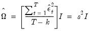 |
(21.10) |
and
 |
(21.11) |
where  is the standard degree-of-freedom corrected estimator of the residual variance.
We may instead employ robust estimators of the coefficient variance  which relax the assumptions of heteroskedasticity and/or zero correlation. Broadly speaking, EViews offers three classes of robust variance estimators that are:
• Robust in the presence of heteroskedasticity. Estimators in this first class are termed Heteroskedasticity Consistent (HC) Covariance estimators.
• Robust in the presence of correlation between observations in different groups or clusters. This second class consists of the family of Cluster Robust (CR) variance estimators.
• Robust in the presence of heteroskedasticity and serial correlation. Estimators in the third class are referred to as Heteroskedasticity and Autocorrelation Consistent Covariance (HAC) estimators.
All of these estimators are special cases of sandwich estimators of the coefficient covariances. The name follows from the structure of the estimators in which different estimates of  are sandwiched between two instances of an outer moment matrix.
It is worth emphasizing all three of these approaches alter the estimates of the coefficient standard errors of an equation but not the point estimates themselves.
Lastly, our discussion here focuses on the linear model. The extension to nonlinear regression is described in
“Nonlinear Least Squares”.
Heteroskedasticity Consistent Covariances
First, we consider coefficient covariance estimators that are robust to the presence of heteroskedasticity.
We divide our discussion of HC covariance estimation into two groups: basic estimators, consisting of White (1980) and degree-of-freedom corrected White (Davidson and MacKinnon 1985), and more general estimators that account for finite samples by adjusting the weights given to residuals on the basis of leverage (Long and Ervin, 2000; Cribari-Neto and da Silva, 2011).
Basic HC Estimators
White (1980) derives a heteroskedasticity consistent covariance matrix estimator which provides consistent estimates of the coefficient covariances in the presence of (conditional) heteroskedasticity of unknown form, where
 |
(21.12) |
Recall that the coefficient variance in question is

Under the basic White approach. we estimate the central matrix  using either the d.f. corrected form
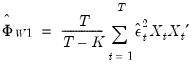 |
(21.13) |
or the uncorrected form
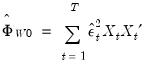 |
(21.14) |
The estimator of  is then used to form the heteroskedasticity consistent coefficient covariance estimator. For example, the degree-of-freedom White heteroskedasticity consistent covariance matrix estimator is given by
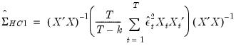 |
(21.15) |
Estimates using this approach are typically referred to as White or Huber-White or (for the d.f. corrected case) White-Hinkley covariances and standard errors.
Example
To illustrate the computation of White covariance estimates in EViews, we employ an example from Wooldridge (2000, p. 251) of an estimate of a wage equation for college professors. The equation uses dummy variables to examine wage differences between four groups of individuals: married men (MARRMALE), married women (MARRFEM), single women (SINGLEFEM), and the base group of single men. The explanatory variables include levels of education (EDUC), experience (EXPER) and tenure (TENURE). The data are in the workfile “Wooldridge.WF1”.

To select the White covariance estimator, specify the equation as before, then select the tab and select in the drop-down. You may, if desired, use the checkbox to remove the default , but in this example, we will use the default setting. (Note that the combo setting is not important in linear specifications).
The output for the robust covariances for this regression are shown below:
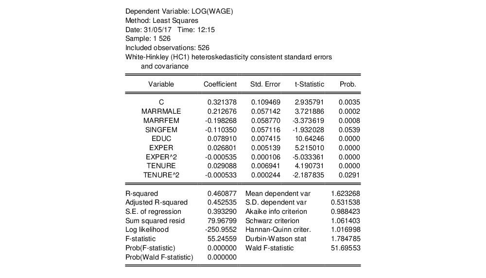
As Wooldridge notes, the heteroskedasticity robust standard errors for this specification are not very different from the non-robust forms, and the test statistics for statistical significance of coefficients are generally unchanged. While robust standard errors are often larger than their usual counterparts, this is not necessarily the case, and indeed in this example, there are some robust standard errors that are smaller than their conventional counterparts.
Notice that EViews reports both the conventional residual-based F-statistic and associated probability and the robust Wald test statistic and p-value for the hypothesis that all non-intercept coefficients are equal to zero.
Recall that the familiar residual F-statistic for testing the null hypothesis depends only on the coefficient point estimates, and not their standard error estimates, and is valid only under the maintained hypotheses of no heteroskedasticity or serial correlation. For ordinary least squares with conventionally estimated standard errors, this statistic is numerically identical to the Wald statistic. When robust standard errors are employed, the numerical equivalence between the two breaks down, so EViews reports both the non-robust conventional residual and the robust Wald F-statistics.
EViews reports the robust F-statistic as the Wald F-statistic in equation output, and the corresponding p-value as Prob(Wald F-statistic). In this example, both the non-robust F-statistic and the robust Wald show that the non-intercept coefficients are jointly statistically significant.
Alternative HC Estimators
The two familiar White covariance estimators described in
“Basic HC Estimators” are two elements of a wider class of HC methods (Long and Ervin, 2000; Cribari-Neto and da Silva, 2011).
This general class of heteroskedasticity consistent sandwich covariance estimators may be written as:
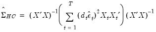 |
(21.16) |
where  are observation-specific weights that are chosen to improve finite sample performance.
EViews allows you to estimate your covariances using several choices for  . In addition to the standard White covariance estimators from above, EViews supports the bias-correcting HC2, pseudo-jackknife HC3 (MacKinnon and White, 1985), and the leverage weighting HC4, HC4m, and HC5 (Cribari-Neto, 2004; Cribaro-Neto and da Silva, 2011; Cribari-Neto, Souza, and Vasconcellos, 2007 and 2008).
The weighting functions for the various HC estimators supported by EViews are provided below:
|
Method |
|
|
HC0 – White |
1 |
|
HC1 – White with d.f. correction |
|
|
HC2 – bias corrected |
|
|
HC3 – pseudo-jackknife |
|
|
HC4 – relative leverage |
|
|
HC4m |
|
|
HC5 |
|
|
User – user-specified |
arbitrary |


where 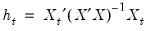 are the diagonal elements of the familiar “hat matrix”
 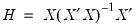 .
.
Note that the HC0 and HC1 methods correspond to the basic White estimators outlined earlier.
Note that HC4, HC4m, and HC5 all depend on an exponential discounting factor  that differs across methods:
• For HC4,
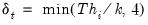
is a truncated function of the ratio between  and the mean
  (Cribari-Neto, 2004; p. 230).
• For HC4m,

where  and
and  are pre-specified parameters (Cribari-Neto and da Silva, 2011). Following Cribari-Neto and da Silva,
EViews chooses default values of  and
and  .
.
• For HC5,

is similar to the HC4 version of  , but with observation specific truncation that depends on the maximal leverage and a pre-specified parameter
  (Cribari-Neto, Souza, and Vasconcellos, 2007 and 2008).
EViews employs a default value of  .
.
Lastly, to allow for maximum flexibility, EViews allows you to provide user-specified  in the form of a series containing those values.
Each of the weight choices modifies the effects of high leverage observations on the calculation of the covariance. See Cribari-Neto (2004), Cribari-Neto and da Silva (2011), and Cribari-Neto, Souza, and Vasconcellos (2007, 2008) for discussion of the effects of these choices.
Note that the full set of HC estimators is only available for linear regression models. For nonlinear regression models, the leverage based methods are not available and only user-specified may be computed.
Example
To illustrate the use of the alternative HC estimators, we continue with the Wooldridge example (
“Example”) considered above. We specify the equation variables as before, then select the tab and click on the drop-down and select :
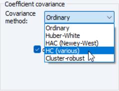
The dialog will change to show you additional options for selecting the :
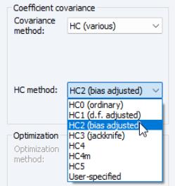
Note that the and items replicate the option from the original dropdown and are included in this list for completeness. If desired, change the method from the default , and if necessary, specify values for the parameters. For example, if you select User-specified, you will be prompted to provide the name of a series in the workfile containing the values of the weights  .
.
Continuing with our example, we use the dropdown to select the method, and retain the default value  . Click on to estimate the model with these settings producing the following results:
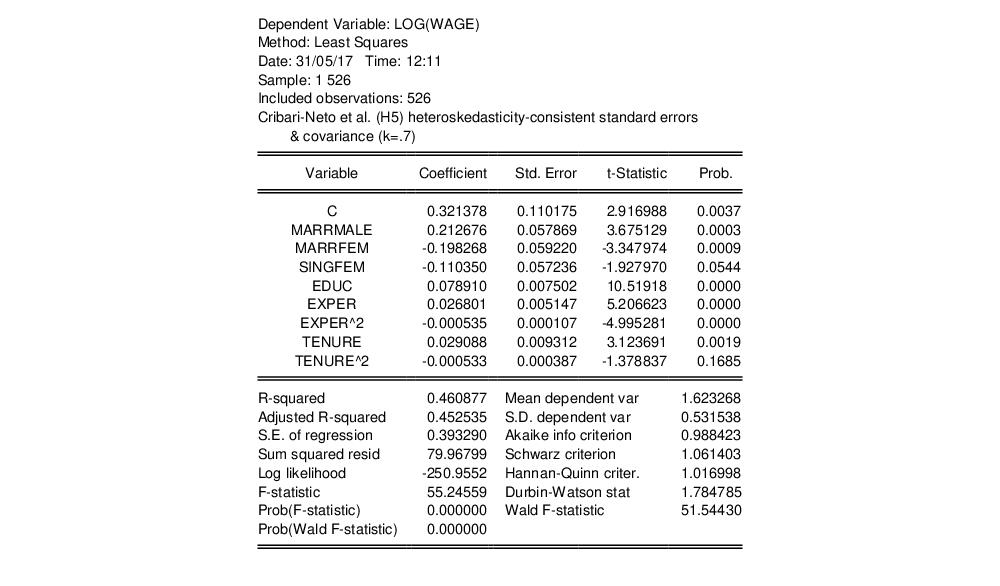
The effects on statistical inference resulting from a different HC estimator are minor, though the quadratic effect of TENURE is no longer significant at conventional test levels.
Cluster-Robust Covariances
In many settings, observations may be grouped into different groups or “clusters” where errors are correlated for observations in the same cluster and uncorrelated for observations in different clusters. EViews offers support for consistent estimation of coefficient covariances that are robust to either one and two-way clustering.
We begin with a single clustering classifier and assume that
 |
(21.17) |
As with the HC and HAC estimators, the cluster-robust estimator is based upon a sandwich form with an estimator the central matrix  :
:
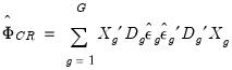 |
(21.18) |
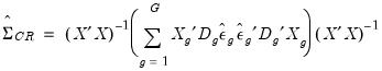 |
(21.19) |
The EViews supported weighting functions for the various CR estimators are analogues to those available for HC estimation:
|
Method |
|
|
CR0 – Ordinary |
1 |
|
CR1 – finite sample corrected (default) |
|
|
CR2 – bias corrected |
|
|
CR3 – pseudo-jackknife |
|
|
CR4 – relative leverage |
|
|
CR4m |
|
|
CR5 |
|
|
User – user-specified |
arbitrary |

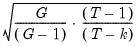


Note that the EViews CR3 differs slightly from the CR3 described by CM in not including the  factor, and that we have defined the CR4, CR4m and CR5 estimators which employ weights that are analogues to those defined for HC covariance estimation.
We may easily extend the robust variance calculation to two-way clustering to handle cases where observations are correlated within two different clustering dimensions (Petersen 2009, Thompson 2011, Cameron, Gelbach, and Miller 2015).
It is easily shown that the variance estimator for clustering by  and
and  may be written as:
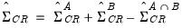 |
(21.20) |
where the  is used to indicate the estimator obtained assuming clustering along the given dimension. Thus, the estimator is formed by adding the covariances obtained by clustering along each of the two dimensions individually, and subtracting off the covariance obtained by defining clusters for the intersection of the two dimensions.
Note that EViews does not perform the eigenvalue adjustment in cases where the resulting estimate is not positive semidefinite.
If you elect to compute cluster-robust covariance estimates, EViews will adjust the t-statistic probabilities in the main estimation output to account for the clustering and will note this adjustment in the output comments. Following Cameron and Miller (CM, 2015), the probabilities are computed using the t-distribution with  degrees-of-freedom in the one-way cluster case, and by
 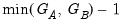 degrees-of-freedom under two-way clustering. Bear in mind that CM note that even with these adjustments, the tests tend to overreject the null.
Furthermore, when cluster-robust covariances are computed, EViews will not display the residual-based F-statistic for the test of significance of the non-intercept regressors. The robust Wald-based F-statistic will be displayed.
Example
We illustrate the computation of cluster-robust covariance estimation in EViews using the test data provided by Petersen via his website:
The data are provided as an EViews workfile “Petersen_cluster.WF1”. There are 5000 observations on four variables in the workfile, the dependent variable Y, independent variable X, and two cluster variables, a firm identifier (FIRMID), and time identifier (YEAR). There are 500 firms, and 10 periods in the balanced design.
First, create the equation object in EViews by selecting or from the main menu, or simply type the keyword equation in the command window. Enter, the regression specification “Y C X” in the edit field, and click on to estimate the equation using standard covariance settings.
The results of this estimation are given below:
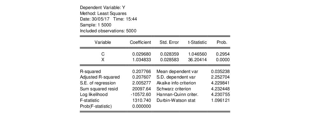
Next, to estimate the equation with FIRMID cluster-robust covariances, click on the button on the equation toolbar to display the estimation dialog, and then click on the tab to show the options.
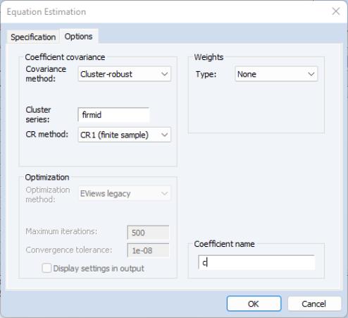
Select in the dropdown, enter “FIRMID” in the edit field, and select a . Here, we choose the method which employs a simple d.f. style adjustment to the basic cluster covariance estimate. Click on to estimate the equation using these settings.
The results are displayed below:
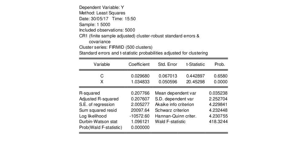
The top portion of the equation output describes both the cluster method (CR1) and the cluster series (FIRMID), along with the number of clusters (500) observed in the estimation sample. In addition, EViews indicates that the reported coefficient standard errors, and t-statistic probabilities have been adjusted for the clustering. As noted earlier, the probabilities are computed using the t-distribution with  degrees-of-freedom.
Note also that EViews no longer displays the ordinary F-statistic and associated probability, but instead shows the robust Wald F-statistic and probability.
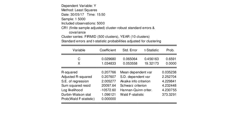
For two-way clustering, we create an equation with the same regression specification, click on the tab, and enter the two cluster series identifiers “FIRMID YEAR” in the edit field. Leaving the remaining options at their current settings, click on to compute and display the estimation results:
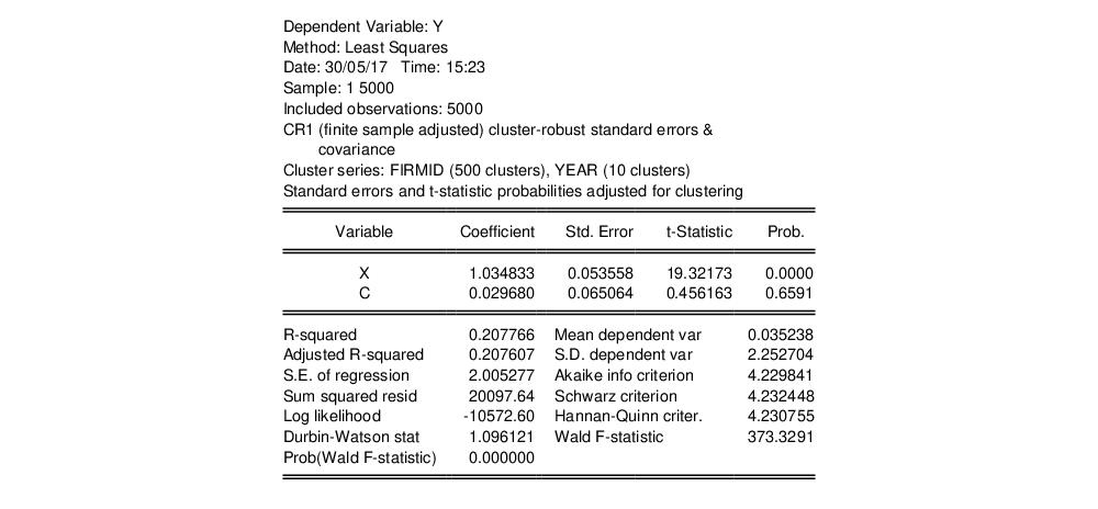
The output shows that the cluster-robust covariance computation is now based on two-way clustering using the 500 clusters in FIRMID and the 10 clusters in YEAR. The t-statistic probabilities are now based on the t-distribution with  degrees-of-freedom.
Notice in all of these examples that the coefficient point estimates and basic fit measures are unchanged. The only changes in results are in the estimated standard errors, and the associated t-statistics, probabilities, and the F-statistics and probabilities.
Lastly, we note that the standard errors and corresponding statistics in the EViews two-way results differ slightly from those reported on the Petersen website. These differences appear to be the result of slightly different finite sample adjustments in the computation of the three individual matrices used to compute the two-way covariance. When you select the CR1 method, EViews adjusts each of the three matrices using the CR1 finite sample adjustment; Petersen’s example appears to apply CR1 to the one-way cluster covariances, while the joint two-way cluster results are computing using CR0.
HAC Consistent Covariances (Newey-West)
The White covariance matrix described above assumes that the residuals of the estimated equation are serially uncorrelated.
Newey and West (1987b) propose a covariance estimator that is consistent in the presence of both heteroskedasticity and autocorrelation (HAC) of unknown form, under the assumption that the autocorrelations between distant observations die out. NW advocate using kernel methods to form an estimate of the long-run variance, 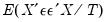 .
.
EViews incorporates and extends the Newey-West approach by allowing you to estimate the HAC consistent coefficient covariance estimator given by:
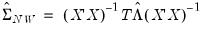 |
(21.21) |
where  is any of the LRCOV estimators described in
Appendix F. “Long-run Covariance Estimation”.
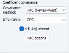
To use the Newey-West HAC method, select the tab and select in the drop-down. As before, you may use the checkbox to remove the default .
Press the button to change the options for the LRCOV estimate.
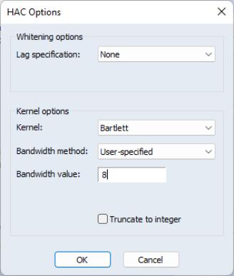
We illustrate the computation of HAC covariances using an example from Stock and Watson (2007, p. 620). In this example, the percentage change of the price of orange juice is regressed upon a constant and the number of days the temperature in Florida reached zero for the current and previous 18 months, using monthly data from 1950 to 2000 The data are in the workfile “Stock_wat.WF1”.
Stock and Watson report Newey-West standard errors computed using a non pre-whitened Bartlett Kernel with a user-specified bandwidth of 8 (note that the bandwidth is equal to one plus what Stock and Watson term the “truncation parameter”  ).
).
The results of this estimation are shown below:
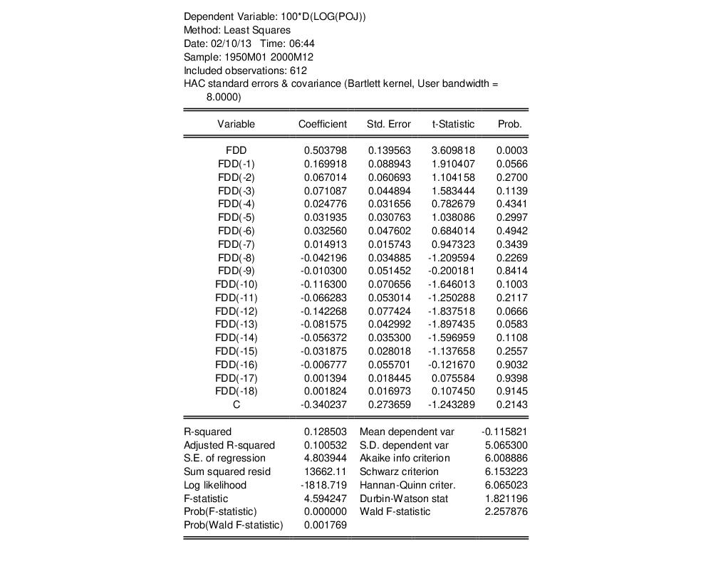
Note in particular that the top of the equation output documents the use of HAC covariance estimates along with relevant information about the settings used to compute the long-run covariance matrix.
The HAC robust Wald p-value is slightly higher than the corresponding non-robust F-statistic p-value, but are significant at conventional test levels.
with tags
heteroskedasticity
t-test
F-test
robust-error
—
Although heteroskedasticity does not produce biased OLS estimates, it leads to a bias in the variance-covariance matrix. This means that standard model testing methods such as t tests or F tests cannot be relied on any longer. This post provides an intuitive illustration of heteroskedasticity and covers the calculation of standard errors that are robust to it.
Data
A popular illustration of heteroskedasticity is the relationship between saving and income, which is shown in the following graph. The dataset is contained the wooldridge package.1
# Load packages
library(dplyr)
library(ggplot2)
library(wooldridge)

# Load the sample
data("saving")

# Only use positive values of saving, which are smaller than income
saving <- saving %>%
  filter(sav > 0,
         inc < 20000,
         sav < inc)

# Plot
ggplot(saving, aes(x = inc, y = sav)) +
  geom_point() +
  geom_smooth(method = "lm", se = FALSE) +
  labs(x = "Annual income", y = "Annual savings")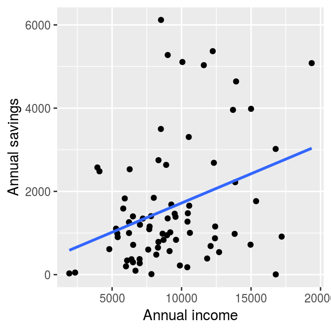
The regression line in the graph shows a clear positive relationship between saving and income. However, as income increases, the differences between the observations and the regression line become larger. This means that there is higher uncertainty about the estimated relationship between the two variables at higher income levels. This is an example of heteroskedasticity.
Since standard model testing methods rely on the assumption that there is no correlation between the independent variables and the variance of the dependent variable, the usual standard errors are not very reliable in the presence of heteroskedasticity. Fortunately, the calculation of robust standard errors can help to mitigate this problem.
Robust standard errors
The regression line above was derived from the model \[sav_i = \beta_0 + \beta_1 inc_i + \epsilon_i,\] for which the following code produces the standard R output:
# Estimate the model
model <- lm(sav ~ inc, data = saving)

# Print estimates and standard test statistics
summary(model)
##
## Call:
## lm(formula = sav ~ inc, data = saving)
##
## Residuals:
## Min 1Q Median 3Q Max
## -2667.8 -874.5 -302.7 431.1 4606.6
##
## Coefficients:
## Estimate Std. Error t value Pr(>|t|)
## (Intercept) 316.19835 462.06882 0.684 0.49595
## inc 0.14052 0.04672 3.007 0.00361 **
## ---
## Signif. codes: 0 '***' 0.001 '**' 0.01 '*' 0.05 '.' 0.1 ' ' 1
##
## Residual standard error: 1413 on 73 degrees of freedom
## Multiple R-squared: 0.1102, Adjusted R-squared: 0.09805
## F-statistic: 9.044 on 1 and 73 DF, p-value: 0.003613t test
Since we already know that the model above suffers from heteroskedasticity, we want to obtain heteroskedasticity robust standard errors and their corresponding t values. In R the function coeftest from the lmtest package can be used in combination with the function vcovHC from the sandwich package to do this.
The first argument of the coeftest function contains the output of the lm function and calculates the t test based on the variance-covariance matrix provided in the vcov argument. The vcovHC function produces that matrix and allows to obtain several types of heteroskedasticity robust versions of it. In our case we obtain a simple White standard error, which is indicated by type = "HC0". Other, more sophisticated methods are described in the documentation of the function, ?vcovHC.
# Load libraries
library("lmtest")
library("sandwich")

# Robust t test
coeftest(model, vcov = vcovHC(model, type = "HC0"))
##
## t test of coefficients:
##
## Estimate Std. Error t value Pr(>|t|)
## (Intercept) 316.198354 414.728032 0.7624 0.448264
## inc 0.140515 0.048805 2.8791 0.005229 **
## ---
## Signif. codes: 0 '***' 0.001 '**' 0.01 '*' 0.05 '.' 0.1 ' ' 1F test
In the post on hypothesis testing the F test is presented as a method to test the joint significance of multiple regressors. The following example adds two new regressors on education and age to the above model and calculates the corresponding (non-robust) F test using the anova function.
# Estimate unrestricted model
model_unres <- lm(sav ~ inc + size + educ + age, data = saving)

# F test
anova(model, model_unres)
## Analysis of Variance Table
##
## Model 1: sav ~ inc
## Model 2: sav ~ inc + size + educ + age
## Res.Df RSS Df Sum of Sq F Pr(>F)
## 1 73 145846877
## 2 70 144286605 3 1560272 0.2523 0.8594For a heteroskedasticity robust F test we perform a Wald test using the waldtest function, which is also contained in the lmtest package. It can be used in a similar way as the anova function, i.e., it uses the output of the restricted and unrestricted model and the robust variance-covariance matrix as argument vcov. Based on the variance-covariance matrix of the unrestriced model we, again, calculate White standard errors.
waldtest(model, model_unres, vcov = vcovHC(model_unres, type = "HC0"))## Wald test
##
## Model 1: sav ~ inc
## Model 2: sav ~ inc + size + educ + age
## Res.Df Df F Pr(>F)
## 1 73
## 2 70 3 0.3625 0.7803Literature
Kennedy, P. (2014). A Guide to Econometrics. Malden (Mass.): Blackwell Publishing 6th ed.