Pytorch матрица ошибок - Решение и исправление самых разных ошибок на TopOshibok.ru

Module Interface¶

class torchmetrics.ConfusionMatrix(**kwargs)[source]¶

Compute the confusion matrix.

This function is a simple wrapper to get the task specific versions of this metric, which is done by setting the
task argument to either 'binary', 'multiclass' or multilabel. See the documentation of
BinaryConfusionMatrix,
MulticlassConfusionMatrix and
MultilabelConfusionMatrix for the specific details of each argument influence
and examples.

Legacy Example:

>>> from torch import tensor
>>> target = tensor([1, 1, 0, 0])
>>> preds = tensor([0, 1, 0, 0])
>>> confmat = ConfusionMatrix(task="binary", num_classes=2)
>>> confmat(preds, target)
tensor([[2, 0],
        [1, 1]])

>>> target = tensor([2, 1, 0, 0])
>>> preds = tensor([2, 1, 0, 1])
>>> confmat = ConfusionMatrix(task="multiclass", num_classes=3)
>>> confmat(preds, target)
tensor([[1, 1, 0],
        [0, 1, 0],
        [0, 0, 1]])

>>> target = tensor([[0, 1, 0], [1, 0, 1]])
>>> preds = tensor([[0, 0, 1], [1, 0, 1]])
>>> confmat = ConfusionMatrix(task="multilabel", num_labels=3)
>>> confmat(preds, target)
tensor([[[1, 0], [0, 1]],
        [[1, 0], [1, 0]],
        [[0, 1], [0, 1]]])

static __new__(cls, task, threshold=0.5, num_classes=None, num_labels=None, normalize=None, ignore_index=None, validate_args=True, **kwargs)[source]¶

Initialize task metric.

Return type:: Metric

BinaryConfusionMatrix¶

class torchmetrics.classification.BinaryConfusionMatrix(threshold=0.5, ignore_index=None, normalize=None, validate_args=True, **kwargs)[source]¶

Compute the confusion matrix for binary tasks.

The confusion matrix \(C\) is constructed such that \(C_{i, j}\) is equal to the number of observations
known to be in class \(i\) but predicted to be in class \(j\). Thus row indices of the confusion matrix
correspond to the true class labels and column indices correspond to the predicted class labels.

For binary tasks, the confusion matrix is a 2×2 matrix with the following structure:

\(C_{0, 0}\): True negatives
\(C_{0, 1}\): False positives
\(C_{1, 0}\): False negatives
\(C_{1, 1}\): True positives

As input to forward and update the metric accepts the following input:

preds (Tensor): An int or float tensor of shape (N, ...). If preds is a floating point
tensor with values outside [0,1] range we consider the input to be logits and will auto apply sigmoid per
element. Addtionally, we convert to int tensor with thresholding using the value in threshold.
target (Tensor): An int tensor of shape (N, ...).

As output to forward and compute the metric returns the following output:

confusion_matrix (Tensor): A tensor containing a (2, 2) matrix

Additional dimension ... will be flattened into the batch dimension.

Parameters:

threshold¶ (float) – Threshold for transforming probability to binary (0,1) predictions
ignore_index¶ (Optional[int]) – Specifies a target value that is ignored and does not contribute to the metric calculation
normalize¶ (Optional[Literal['true', 'pred', 'all', 'none']]) –

Normalization mode for confusion matrix. Choose from:
- None or 'none': no normalization (default)
- 'true': normalization over the targets (most commonly used)
- 'pred': normalization over the predictions
- 'all': normalization over the whole matrix
validate_args¶ (bool) – bool indicating if input arguments and tensors should be validated for correctness.
Set to False for faster computations.
kwargs¶ (Any) – Additional keyword arguments, see Advanced metric settings for more info.

Example (preds is int tensor):

>>> from torchmetrics.classification import BinaryConfusionMatrix
>>> target = torch.tensor([1, 1, 0, 0])
>>> preds = torch.tensor([0, 1, 0, 0])
>>> bcm = BinaryConfusionMatrix()
>>> bcm(preds, target)
tensor([[2, 0],
        [1, 1]])

Example (preds is float tensor):

>>> from torchmetrics.classification import BinaryConfusionMatrix
>>> target = torch.tensor([1, 1, 0, 0])
>>> preds = torch.tensor([0.35, 0.85, 0.48, 0.01])
>>> bcm = BinaryConfusionMatrix()
>>> bcm(preds, target)
tensor([[2, 0],
        [1, 1]])

plot(val=None, ax=None, add_text=True, labels=None)[source]¶

Plot a single or multiple values from the metric.

Parameters:

val¶ (Optional[Tensor]) – Either a single result from calling metric.forward or metric.compute or a list of these results.
If no value is provided, will automatically call metric.compute and plot that result.
ax¶ (Optional[Axes]) – An matplotlib axis object. If provided will add plot to that axis
add_text¶ (bool) – if the value of each cell should be added to the plot
labels¶ (Optional[List[str]]) – a list of strings, if provided will be added to the plot to indicate the different classes

Return type:

Tuple[Figure, Union[Axes, ndarray]]

Returns:

Figure and Axes object

Raises:

ModuleNotFoundError – If matplotlib is not installed

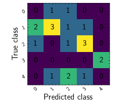
>>> from torch import randint
>>> from torchmetrics.classification import MulticlassConfusionMatrix
>>> metric = MulticlassConfusionMatrix(num_classes=5)
>>> metric.update(randint(5, (20,)), randint(5, (20,)))
>>> fig_, ax_ = metric.plot()

MulticlassConfusionMatrix¶

class torchmetrics.classification.MulticlassConfusionMatrix(num_classes, ignore_index=None, normalize=None, validate_args=True, **kwargs)[source]¶

Compute the confusion matrix for multiclass tasks.

For multiclass tasks, the confusion matrix is a NxN matrix, where:

\(C_{i, i}\) represents the number of true positives for class \(i\)
\(\sum_{j=1, j\neq i}^N C_{i, j}\) represents the number of false negatives for class \(i\)
\(\sum_{i=1, i\neq j}^N C_{i, j}\) represents the number of false positives for class \(i\)
the sum of the remaining cells in the matrix represents the number of true negatives for class \(i\)

As input to forward and update the metric accepts the following input:

preds (Tensor): An int or float tensor of shape (N, ...). If preds is a floating point
tensor with values outside [0,1] range we consider the input to be logits and will auto apply sigmoid per
element. Addtionally, we convert to int tensor with thresholding using the value in threshold.
target (Tensor): An int tensor of shape (N, ...).

As output to forward and compute the metric returns the following output:

confusion_matrix: [num_classes, num_classes] matrix

Parameters:

num_classes¶ (int) – Integer specifing the number of classes
ignore_index¶ (Optional[int]) – Specifies a target value that is ignored and does not contribute to the metric calculation
normalize¶ (Optional[Literal['true', 'pred', 'all', 'none']]) –

Normalization mode for confusion matrix. Choose from:
- None or 'none': no normalization (default)
- 'true': normalization over the targets (most commonly used)
- 'pred': normalization over the predictions
- 'all': normalization over the whole matrix
validate_args¶ (bool) – bool indicating if input arguments and tensors should be validated for correctness.
Set to False for faster computations.
kwargs¶ (Any) – Additional keyword arguments, see Advanced metric settings for more info.

Example (pred is integer tensor):

>>> from torch import tensor
>>> from torchmetrics.classification import MulticlassConfusionMatrix
>>> target = tensor([2, 1, 0, 0])
>>> preds = tensor([2, 1, 0, 1])
>>> metric = MulticlassConfusionMatrix(num_classes=3)
>>> metric(preds, target)
tensor([[1, 1, 0],
        [0, 1, 0],
        [0, 0, 1]])

Example (pred is float tensor):

>>> from torchmetrics.classification import MulticlassConfusionMatrix
>>> target = tensor([2, 1, 0, 0])
>>> preds = tensor([[0.16, 0.26, 0.58],
...                 [0.22, 0.61, 0.17],
...                 [0.71, 0.09, 0.20],
...                 [0.05, 0.82, 0.13]])
>>> metric = MulticlassConfusionMatrix(num_classes=3)
>>> metric(preds, target)
tensor([[1, 1, 0],
        [0, 1, 0],
        [0, 0, 1]])

plot(val=None, ax=None, add_text=True, labels=None)[source]¶

Plot a single or multiple values from the metric.

Parameters:

val¶ (Optional[Tensor]) – Either a single result from calling metric.forward or metric.compute or a list of these results.
If no value is provided, will automatically call metric.compute and plot that result.
ax¶ (Optional[Axes]) – An matplotlib axis object. If provided will add plot to that axis
add_text¶ (bool) – if the value of each cell should be added to the plot
labels¶ (Optional[List[str]]) – a list of strings, if provided will be added to the plot to indicate the different classes

Return type:

Tuple[Figure, Union[Axes, ndarray]]

Returns:

Figure and Axes object

Raises:

ModuleNotFoundError – If matplotlib is not installed

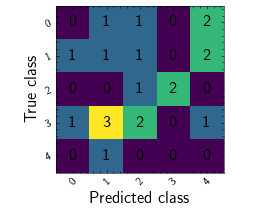
>>> from torch import randint
>>> from torchmetrics.classification import MulticlassConfusionMatrix
>>> metric = MulticlassConfusionMatrix(num_classes=5)
>>> metric.update(randint(5, (20,)), randint(5, (20,)))
>>> fig_, ax_ = metric.plot()

MultilabelConfusionMatrix¶

class torchmetrics.classification.MultilabelConfusionMatrix(num_labels, threshold=0.5, ignore_index=None, normalize=None, validate_args=True, **kwargs)[source]¶

Compute the confusion matrix for multilabel tasks.

For multilabel tasks, the confusion matrix is a Nx2x2 tensor, where each 2×2 matrix corresponds to the confusion
for that label. The structure of each 2×2 matrix is as follows:

\(C_{0, 0}\): True negatives
\(C_{0, 1}\): False positives
\(C_{1, 0}\): False negatives
\(C_{1, 1}\): True positives

As input to ‘update’ the metric accepts the following input:

preds (int or float tensor): (N, C, ...). If preds is a floating point tensor with values outside
[0,1] range we consider the input to be logits and will auto apply sigmoid per element. Addtionally,
we convert to int tensor with thresholding using the value in threshold.
target (int tensor): (N, C, ...)

As output of ‘compute’ the metric returns the following output:

confusion matrix: [num_labels,2,2] matrix

Parameters:

num_classes¶ – Integer specifing the number of labels
threshold¶ (float) – Threshold for transforming probability to binary (0,1) predictions
ignore_index¶ (Optional[int]) – Specifies a target value that is ignored and does not contribute to the metric calculation
normalize¶ (Optional[Literal['true', 'pred', 'all', 'none']]) –

Normalization mode for confusion matrix. Choose from:
- None or 'none': no normalization (default)
- 'true': normalization over the targets (most commonly used)
- 'pred': normalization over the predictions
- 'all': normalization over the whole matrix
validate_args¶ (bool) – bool indicating if input arguments and tensors should be validated for correctness.
Set to False for faster computations.
kwargs¶ (Any) – Additional keyword arguments, see Advanced metric settings for more info.

Example (preds is int tensor):

>>> from torch import tensor
>>> from torchmetrics.classification import MultilabelConfusionMatrix
>>> target = tensor([[0, 1, 0], [1, 0, 1]])
>>> preds = tensor([[0, 0, 1], [1, 0, 1]])
>>> metric = MultilabelConfusionMatrix(num_labels=3)
>>> metric(preds, target)
tensor([[[1, 0], [0, 1]],
        [[1, 0], [1, 0]],
        [[0, 1], [0, 1]]])

Example (preds is float tensor):

>>> from torchmetrics.classification import MultilabelConfusionMatrix
>>> target = tensor([[0, 1, 0], [1, 0, 1]])
>>> preds = tensor([[0.11, 0.22, 0.84], [0.73, 0.33, 0.92]])
>>> metric = MultilabelConfusionMatrix(num_labels=3)
>>> metric(preds, target)
tensor([[[1, 0], [0, 1]],
        [[1, 0], [1, 0]],
        [[0, 1], [0, 1]]])

plot(val=None, ax=None, add_text=True, labels=None)[source]¶

Plot a single or multiple values from the metric.

Parameters:

val¶ (Optional[Tensor]) – Either a single result from calling metric.forward or metric.compute or a list of these results.
If no value is provided, will automatically call metric.compute and plot that result.
ax¶ (Optional[Axes]) – An matplotlib axis object. If provided will add plot to that axis
add_text¶ (bool) – if the value of each cell should be added to the plot
labels¶ (Optional[List[str]]) – a list of strings, if provided will be added to the plot to indicate the different classes

Return type:

Tuple[Figure, Union[Axes, ndarray]]

Returns:

Figure and Axes object

Raises:

ModuleNotFoundError – If matplotlib is not installed

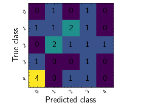
>>> from torch import randint
>>> from torchmetrics.classification import MulticlassConfusionMatrix
>>> metric = MulticlassConfusionMatrix(num_classes=5)
>>> metric.update(randint(5, (20,)), randint(5, (20,)))
>>> fig_, ax_ = metric.plot()

Functional Interface¶

confusion_matrix¶

torchmetrics.functional.confusion_matrix(preds, target, task, threshold=0.5, num_classes=None, num_labels=None, normalize=None, ignore_index=None, validate_args=True)[source]¶

Compute the confusion matrix.

This function is a simple wrapper to get the task specific versions of this metric, which is done by setting the
task argument to either 'binary', 'multiclass' or multilabel. See the documentation of
binary_confusion_matrix(),
multiclass_confusion_matrix() and
multilabel_confusion_matrix() for
the specific details of each argument influence and examples.

Return type:: Tensor

Legacy Example:

>>> from torch import tensor
>>> from torchmetrics.classification import ConfusionMatrix
>>> target = tensor([1, 1, 0, 0])
>>> preds = tensor([0, 1, 0, 0])
>>> confmat = ConfusionMatrix(task="binary")
>>> confmat(preds, target)
tensor([[2, 0],
        [1, 1]])

>>> target = tensor([2, 1, 0, 0])
>>> preds = tensor([2, 1, 0, 1])
>>> confmat = ConfusionMatrix(task="multiclass", num_classes=3)
>>> confmat(preds, target)
tensor([[1, 1, 0],
        [0, 1, 0],
        [0, 0, 1]])

>>> target = tensor([[0, 1, 0], [1, 0, 1]])
>>> preds = tensor([[0, 0, 1], [1, 0, 1]])
>>> confmat = ConfusionMatrix(task="multilabel", num_labels=3)
>>> confmat(preds, target)
tensor([[[1, 0], [0, 1]],
        [[1, 0], [1, 0]],
        [[0, 1], [0, 1]]])

binary_confusion_matrix¶

torchmetrics.functional.classification.binary_confusion_matrix(preds, target, threshold=0.5, normalize=None, ignore_index=None, validate_args=True)[source]¶

Compute the confusion matrix for binary tasks.

Accepts the following input tensors:

preds (int or float tensor): (N, ...). If preds is a floating point tensor with values outside
[0,1] range we consider the input to be logits and will auto apply sigmoid per element. Addtionally,
we convert to int tensor with thresholding using the value in threshold.
target (int tensor): (N, ...)

Additional dimension ... will be flattened into the batch dimension.

Parameters:

preds¶ (Tensor) – Tensor with predictions
target¶ (Tensor) – Tensor with true labels
threshold¶ (float) – Threshold for transforming probability to binary (0,1) predictions
normalize¶ (Optional[Literal['true', 'pred', 'all', 'none']]) –

Normalization mode for confusion matrix. Choose from:
- None or 'none': no normalization (default)
- 'true': normalization over the targets (most commonly used)
- 'pred': normalization over the predictions
- 'all': normalization over the whole matrix
ignore_index¶ (Optional[int]) – Specifies a target value that is ignored and does not contribute to the metric calculation
validate_args¶ (bool) – bool indicating if input arguments and tensors should be validated for correctness.
Set to False for faster computations.

Return type:

Tensor

Returns:

A [2, 2] tensor

Example (preds is int tensor):

>>> from torch import tensor
>>> from torchmetrics.functional.classification import binary_confusion_matrix
>>> target = tensor([1, 1, 0, 0])
>>> preds = tensor([0, 1, 0, 0])
>>> binary_confusion_matrix(preds, target)
tensor([[2, 0],
        [1, 1]])

Example (preds is float tensor):

>>> from torchmetrics.functional.classification import binary_confusion_matrix
>>> target = tensor([1, 1, 0, 0])
>>> preds = tensor([0.35, 0.85, 0.48, 0.01])
>>> binary_confusion_matrix(preds, target)
tensor([[2, 0],
        [1, 1]])

multiclass_confusion_matrix¶

torchmetrics.functional.classification.multiclass_confusion_matrix(preds, target, num_classes, normalize=None, ignore_index=None, validate_args=True)[source]¶

Compute the confusion matrix for multiclass tasks.

Accepts the following input tensors:

preds: (N, ...) (int tensor) or (N, C, ..) (float tensor). If preds is a floating point
we apply torch.argmax along the C dimension to automatically convert probabilities/logits into
an int tensor.
target (int tensor): (N, ...)

Additional dimension ... will be flattened into the batch dimension.

Parameters:

preds¶ (Tensor) – Tensor with predictions
target¶ (Tensor) – Tensor with true labels
num_classes¶ (int) – Integer specifing the number of classes
normalize¶ (Optional[Literal['true', 'pred', 'all', 'none']]) –

Normalization mode for confusion matrix. Choose from:
- None or 'none': no normalization (default)
- 'true': normalization over the targets (most commonly used)
- 'pred': normalization over the predictions
- 'all': normalization over the whole matrix
ignore_index¶ (Optional[int]) – Specifies a target value that is ignored and does not contribute to the metric calculation
validate_args¶ (bool) – bool indicating if input arguments and tensors should be validated for correctness.
Set to False for faster computations.

Return type:

Tensor

Returns:

A [num_classes, num_classes] tensor

Example (pred is integer tensor):

>>> from torch import tensor
>>> from torchmetrics.functional.classification import multiclass_confusion_matrix
>>> target = tensor([2, 1, 0, 0])
>>> preds = tensor([2, 1, 0, 1])
>>> multiclass_confusion_matrix(preds, target, num_classes=3)
tensor([[1, 1, 0],
        [0, 1, 0],
        [0, 0, 1]])

Example (pred is float tensor):

>>> from torchmetrics.functional.classification import multiclass_confusion_matrix
>>> target = tensor([2, 1, 0, 0])
>>> preds = tensor([[0.16, 0.26, 0.58],
...                 [0.22, 0.61, 0.17],
...                 [0.71, 0.09, 0.20],
...                 [0.05, 0.82, 0.13]])
>>> multiclass_confusion_matrix(preds, target, num_classes=3)
tensor([[1, 1, 0],
        [0, 1, 0],
        [0, 0, 1]])

multilabel_confusion_matrix¶

torchmetrics.functional.classification.multilabel_confusion_matrix(preds, target, num_labels, threshold=0.5, normalize=None, ignore_index=None, validate_args=True)[source]¶

Compute the confusion matrix for multilabel tasks.

Accepts the following input tensors:

preds (int or float tensor): (N, C, ...). If preds is a floating point tensor with values outside
[0,1] range we consider the input to be logits and will auto apply sigmoid per element. Addtionally,
we convert to int tensor with thresholding using the value in threshold.
target (int tensor): (N, C, ...)

Additional dimension ... will be flattened into the batch dimension.

Parameters:

preds¶ (Tensor) – Tensor with predictions
target¶ (Tensor) – Tensor with true labels
num_labels¶ (int) – Integer specifing the number of labels
threshold¶ (float) – Threshold for transforming probability to binary (0,1) predictions
normalize¶ (Optional[Literal['true', 'pred', 'all', 'none']]) –

Normalization mode for confusion matrix. Choose from:
- None or 'none': no normalization (default)
- 'true': normalization over the targets (most commonly used)
- 'pred': normalization over the predictions
- 'all': normalization over the whole matrix
ignore_index¶ (Optional[int]) – Specifies a target value that is ignored and does not contribute to the metric calculation
validate_args¶ (bool) – bool indicating if input arguments and tensors should be validated for correctness.
Set to False for faster computations.

Return type:

Tensor

Returns:

A [num_labels, 2, 2] tensor

Example (preds is int tensor):

>>> from torch import tensor
>>> from torchmetrics.functional.classification import multilabel_confusion_matrix
>>> target = tensor([[0, 1, 0], [1, 0, 1]])
>>> preds = tensor([[0, 0, 1], [1, 0, 1]])
>>> multilabel_confusion_matrix(preds, target, num_labels=3)
tensor([[[1, 0], [0, 1]],
        [[1, 0], [1, 0]],
        [[0, 1], [0, 1]]])

Example (preds is float tensor):

>>> from torchmetrics.functional.classification import multilabel_confusion_matrix
>>> target = tensor([[0, 1, 0], [1, 0, 1]])
>>> preds = tensor([[0.11, 0.22, 0.84], [0.73, 0.33, 0.92]])
>>> multilabel_confusion_matrix(preds, target, num_labels=3)
tensor([[[1, 0], [0, 1]],
        [[1, 0], [1, 0]],
        [[0, 1], [0, 1]]])

Источник

class ignite.metrics.confusion_matrix.ConfusionMatrix(num_classes, average=None, output_transform=<function ConfusionMatrix.<lambda>>, device=device(type=’cpu’))[source]#

Calculates confusion matrix for multi-class data.

update must receive output of the form (y_pred, y).
y_pred must contain logits and has the following shape (batch_size, num_classes, …).
If you are doing binary classification, see Note for an example on how to get this.
y should have the following shape (batch_size, …) and contains ground-truth class indices
with or without the background class. During the computation, argmax of y_pred is taken to determine
predicted classes.

Parameters

num_classes (int) – Number of classes, should be > 1. See notes for more details.
average (Optional[str]) – confusion matrix values averaging schema: None, “samples”, “recall”, “precision”.
Default is None. If average=”samples” then confusion matrix values are normalized by the number of seen
samples. If average=”recall” then confusion matrix values are normalized such that diagonal values
represent class recalls. If average=”precision” then confusion matrix values are normalized such that
diagonal values represent class precisions.
output_transform (Callable) – a callable that is used to transform the
Engine’s process_function’s output into the
form expected by the metric. This can be useful if, for example, you have a multi-output model and
you want to compute the metric with respect to one of the outputs.
device (Union[str, torch.device]) – specifies which device updates are accumulated on. Setting the metric’s
device to be the same as your update arguments ensures the update method is non-blocking. By
default, CPU.

Note

The confusion matrix is formatted such that columns are predictions and rows are targets.
For example, if you were to plot the matrix, you could correctly assign to the horizontal axis
the label “predicted values” and to the vertical axis the label “actual values”.

Note

In case of the targets y in (batch_size, …) format, target indices between 0 and num_classes only
contribute to the confusion matrix and others are neglected. For example, if num_classes=20 and target index
equal 255 is encountered, then it is filtered out.

Examples

For more information on how metric works with Engine, visit Attach Engine API.

from collections import OrderedDict

import torch
from torch import nn, optim

from ignite.engine import *
from ignite.handlers import *
from ignite.metrics import *
from ignite.utils import *
from ignite.contrib.metrics.regression import *
from ignite.contrib.metrics import *

# create default evaluator for doctests

def eval_step(engine, batch):
    return batch

default_evaluator = Engine(eval_step)

# create default optimizer for doctests

param_tensor = torch.zeros([1], requires_grad=True)
default_optimizer = torch.optim.SGD([param_tensor], lr=0.1)

# create default trainer for doctests
# as handlers could be attached to the trainer,
# each test must define his own trainer using `.. testsetup:`

def get_default_trainer():

    def train_step(engine, batch):
        return batch

    return Engine(train_step)

# create default model for doctests

default_model = nn.Sequential(OrderedDict([
    ('base', nn.Linear(4, 2)),
    ('fc', nn.Linear(2, 1))
]))

manual_seed(666)

metric = ConfusionMatrix(num_classes=3)
metric.attach(default_evaluator, 'cm')
y_true = torch.tensor([0, 1, 0, 1, 2])
y_pred = torch.tensor([
    [0.0, 1.0, 0.0],
    [0.0, 1.0, 0.0],
    [1.0, 0.0, 0.0],
    [0.0, 1.0, 0.0],
    [0.0, 1.0, 0.0],
])
state = default_evaluator.run([[y_pred, y_true]])
print(state.metrics['cm'])

tensor([[1, 1, 0],
        [0, 2, 0],
        [0, 1, 0]])

If you are doing binary classification with a single output unit, you may have to transform your network output,
so that you have one value for each class. E.g. you can transform your network output into a one-hot vector
with:

def binary_one_hot_output_transform(output):
    y_pred, y = output
    y_pred = torch.sigmoid(y_pred).round().long()
    y_pred = ignite.utils.to_onehot(y_pred, 2)
    y = y.long()
    return y_pred, y

metric = ConfusionMatrix(num_classes=2, output_transform=binary_one_hot_output_transform)
metric.attach(default_evaluator, 'cm')
y_true = torch.tensor([0, 1, 0, 1, 0])
y_pred = torch.tensor([0, 0, 1, 1, 0])
state = default_evaluator.run([[y_pred, y_true]])
print(state.metrics['cm'])

Methods

`compute`	Computes the metric based on it’s accumulated state.
`normalize`	Normalize given matrix with given average.
`reset`	Resets the metric to it’s initial state.
`update`	Updates the metric’s state using the passed batch output.

compute()[source]#

Computes the metric based on it’s accumulated state.

By default, this is called at the end of each epoch.

Returns: the actual quantity of interest. However, if a Mapping is returned,
it will be (shallow) flattened into engine.state.metrics when
completed() is called.
Return type: Any
Raises: NotComputableError – raised when the metric cannot be computed.

static normalize(matrix, average)[source]#

Normalize given matrix with given average.

Parameters

matrix (torch.Tensor) –
average (str) –

Return type

torch.Tensor

reset()[source]#

Resets the metric to it’s initial state.

By default, this is called at the start of each epoch.

Return type: None

update(output)[source]#

Updates the metric’s state using the passed batch output.

By default, this is called once for each batch.

Parameters: output (Sequence[torch.Tensor]) – the is the output from the engine’s process function.
Return type: None

Источник

PyTorch
May 3, 2023
June 26, 2022

In the real world, often our data has imbalanced classes e.g., 99.9% of observations are of class 1, and only 0.1% are class 2. In the presence of imbalanced classes, accuracy suffers from a paradox where a model is highly accurate but lacks predictive power.

For example, imagine we are trying to predict the presence of a very rare cancer that occurs in 0.1% of the population. After training our model, we find the accuracy is at 95%. However, 99.9% of people do not have cancer. If we simply created a model that predicted that nobody had that form of cancer, our naive model would be 4.9% more accurate, but clearly is not able to predict anything. For this reason, we are often motivated to use other metrics like confusion matrix, precision, recall, and the F 1 score.

When we have balanced classes, accuracy is just like in binary classification, a simple and interpretable choice for an evaluation metric. Accuracy is the number of correct predictions divided by the number of observations and works just as well in multiclass as binary classification. However, when we have imbalanced classes, we should be inclined to use other evaluation metrics.

Confusion matrices are an easy, effective visualization of a classifier’s performance. One of the major benefits of confusion matrices is their interpretability. Each column of the matrix (often visualized as a heatmap) represents predicted classes, while every row shows actual classes. The end result is that every cell is one possible combination of predicted and actual classes.

Predict the model on the test data

We have trained the cifar10 model over 5 epochs on the training dataset. Now we need to check if the network has learned anything at all. We will check this by predicting the class label that the neural network outputs, and checking it against the ground truth.

y_true = []
y_pred = []

for data in tqdm(testloader):
  images,labels=data[0].to(device),data[1]  
  y_true.extend(labels.numpy())

  outputs=model(images)

  _, predicted = torch.max(outputs, 1)
  y_pred.extend(predicted.cpu().numpy())

Although these metrics can be easily computed manually by comparing the actual and predicted class labels, scikit-learn provides a convenient confusion_matrix function that we can use, as follows:

cf_matrix = confusion_matrix(y_true, y_pred)

The array that was returned after executing the code provides us with information about the different types of errors the classifier made on the test dataset.

Now, we can simply total up each type of result, substitute it into the template, and create a confusion matrix that will concisely summarize the results of testing the classifier:

class_names = ('plane', 'car', 'bird', 'cat',
           'deer', 'dog', 'frog', 'horse', 'ship', 'truck')

# Create pandas dataframe
dataframe = pd.DataFrame(cf_matrix, index=class_names, columns=class_names)

We can map this information onto the confusion matrix using Matplotlib. The following confusion matrix plot, with the added labels, should make the results a little bit easier to interpret:

plt.figure(figsize=(8, 6))

# Create heatmap
sns.heatmap(dataframe, annot=True, cbar=None,cmap="YlGnBu",fmt="d")

plt.title("Confusion Matrix"), plt.tight_layout()

plt.ylabel("True Class"), 
plt.xlabel("Predicted Class")
plt.show()

All correct predictions are located in the diagonal of the table (highlighted in blue), so it is easy to visually inspect the table for prediction errors, as values outside the diagonal will represent them.

This is probably best explained using an example. In the Visualizing a Classifier’s Performance solution, the top-left cell is the number of observations predicted to be ‘Plane’.However, the model does not do as well at predicting dog vs cat.

There are three things about confusion matrices. First, a perfect model will have values along the diagonal and zeros everywhere else. A bad model will look like the observation counts will be spread evenly around cells.

Second, a confusion matrix lets us see not only where the model was wrong, but also how it was wrong. That is, we can look at patterns of misclassification. For example, our model had an easy time differentiating ‘truck and dog’, but a much more difficult time classifying ‘dog and cat’.

Finally, confusion matrices work with any number of classes (although if we had one million classes in our target vector, the confusion matrix visualization might be difficult to read).

Split Imbalanced dataset using sklearn Stratified train_test_split().
Calculate Precision, Recall and F1 score for Keras model

Run this code in Google Colab

Источник

As a data scientist or software engineer working with PyTorch, you may find yourself needing to use transfer learning to train a model on a new dataset. Transfer learning allows you to take an existing pre-trained model and fine-tune it for a specific task, rather than training a new model from scratch. In this tutorial, we will explore how to use confusion matrix and test accuracy to evaluate the performance of a transfer learning model in PyTorch.

A Guide to Confusion Matrix and Test Accuracy for PyTorch Transfer Learning Tutorial

What is Transfer Learning?

Transfer learning is a technique used in deep learning where a pre-trained model is used as a starting point for a new task. The pre-trained model has already learned a large amount of information on a different dataset, and this knowledge can be applied to a new dataset. Rather than training a new model from scratch, which can be computationally expensive and time-consuming, transfer learning allows us to take advantage of the pre-trained model’s knowledge and fine-tune it for our specific task.

There are many pre-trained models available for use in PyTorch, such as VGG, ResNet, and Inception. These models have been trained on large datasets such as ImageNet, which contains millions of labeled images. By using transfer learning, we can leverage the pre-trained model’s ability to recognize features in images, which can be applied to our new dataset.

What is a Confusion Matrix?

A confusion matrix is a table that is used to evaluate the performance of a classification model. It shows the number of correct and incorrect predictions made by the model, compared to the actual labels of the data. The confusion matrix has four components:

True positives (TP): The number of correctly predicted positive samples.
False positives (FP): The number of incorrectly predicted positive samples.
True negatives (TN): The number of correctly predicted negative samples.
False negatives (FN): The number of incorrectly predicted negative samples.

A confusion matrix can be represented as follows:

	Actual Positive	Actual Negative
Predicted Positive	True Positive (TP)	False Positive (FP)
Predicted Negative	False Negative (FN)	True Negative (TN)

How to Calculate Test Accuracy?

Test accuracy is a metric used to evaluate the performance of a classification model. It represents the percentage of correctly classified samples in the test set. Test accuracy can be calculated using the following formula:

Test Accuracy = (TP + TN) / (TP + FP + TN + FN)

Evaluating Transfer Learning Model Performance

When using transfer learning, it is important to evaluate the performance of the model on your specific task. One way to do this is by using a confusion matrix and test accuracy.

To evaluate the performance of a transfer learning model, follow these steps:

Load the pre-trained model and fine-tune it on your new dataset.
Split your dataset into training and testing sets.
Use the trained model to make predictions on the test set.
Calculate the confusion matrix and test accuracy.

Here is an example of how to calculate the confusion matrix and test accuracy using PyTorch:

import torch
import torch.nn as nn
import torchvision.models as models
import torchvision.transforms as transforms
import torchvision.datasets as datasets
from sklearn.metrics import confusion_matrix

# Load the pre-trained model
model = models.resnet18(pretrained=True)

# Replace the last fully connected layer with a new one
num_ftrs = model.fc.in_features
model.fc = nn.Linear(num_ftrs, 2)

# Define the loss function and optimizer
criterion = nn.CrossEntropyLoss()
optimizer = torch.optim.SGD(model.parameters(), lr=0.001, momentum=0.9)

# Load the data
data_transforms = {
    'train': transforms.Compose([
        transforms.RandomResizedCrop(224),
        transforms.RandomHorizontalFlip(),
        transforms.ToTensor(),
        transforms.Normalize([0.485, 0.456, 0.406], [0.229, 0.224, 0.225])
    ]),
    'test': transforms.Compose([
        transforms.Resize(256),
        transforms.CenterCrop(224),
        transforms.ToTensor(),
        transforms.Normalize([0.485, 0.456, 0.406], [0.229, 0.224, 0.225])
    ])
}

data_dir = 'path/to/dataset'
image_datasets = {x: datasets.ImageFolder(os.path.join(data_dir, x), data_transforms[x])
                  for x in ['train', 'test']}
dataloaders = {x: torch.utils.data.DataLoader(image_datasets[x], batch_size=4,
                                             shuffle=True, num_workers=4)
              for x in ['train', 'test']}
dataset_sizes = {x: len(image_datasets[x]) for x in ['train', 'test']}

# Make predictions on test set
model.eval()
y_pred = []
y_true = []
with torch.no_grad():
    for inputs, labels in dataloaders['test']:
        inputs = inputs.to(device)
        labels = labels.to(device)
        outputs = model(inputs)
        _, preds = torch.max(outputs, 1)
        y_pred.extend(preds.cpu().numpy())
        y_true.extend(labels.cpu().numpy())

# Calculate confusion matrix
cm = confusion_matrix(y_true, y_pred)

# Calculate test accuracy
test_acc = (cm[0][0] + cm[1][1]) / (cm[0][0] + cm[0][1] + cm[1][0] + cm[1][1])

In this example, we load a pre-trained ResNet18 model and fine-tune it on a new dataset. We then split the dataset into training and testing sets and make predictions on the test set using the trained model. We calculate the confusion matrix using the confusion_matrix function from scikit-learn, and then calculate the test accuracy using the formula discussed earlier.

Conclusion

In this tutorial, we explored how to use confusion matrix and test accuracy to evaluate the performance of a transfer learning model in PyTorch. Transfer learning is a powerful technique that allows us to leverage pre-trained models to train new models on specific tasks. By using a confusion matrix and test accuracy, we can evaluate the performance of our transfer learning model and make improvements as necessary.

About Saturn Cloud

Saturn Cloud is your all-in-one solution for data science & ML development, deployment, and data pipelines in the cloud. Spin up a notebook with 4TB of RAM, add a GPU, connect to a distributed cluster of workers, and more. Join today and get 150 hours of free compute per month.

Источник

pytorch-confusion-matrix

A self-contained PyTorch library for differentiable precision, recall,
F-beta score (including F1 score), and dice coefficient.

The only dependency is PyTorch.

These scores are «the bigger, the better»,
so 1 - score can be used as a loss function.

Our contribution:

Both y_true and y_pred are of shape [N, C, ...], where N is batch size
and C is the number of channels. They must be float tensors.
We allow both input tensors to be real-valued probabilities,
which generalize 0-1 hard labels.
We formally separate different averaging methods
for these metrics, such as macro, micro, samples,
according to sklearn conventions

You can just copy the code without the fuss of importing from this repository.

Источник

Module Interface¶

BinaryConfusionMatrix¶

MulticlassConfusionMatrix¶

MultilabelConfusionMatrix¶

Functional Interface¶

confusion_matrix¶

binary_confusion_matrix¶

multiclass_confusion_matrix¶

multilabel_confusion_matrix¶

Predict the model on the test data

Related Post

Run this code in Google Colab

A Guide to Confusion Matrix and Test Accuracy for PyTorch Transfer Learning Tutorial

What is Transfer Learning?

What is a Confusion Matrix?

How to Calculate Test Accuracy?

Evaluating Transfer Learning Model Performance

Conclusion

About Saturn Cloud

pytorch-confusion-matrix