Эту функцию называют также «логлосс» (logloss / log_loss), перекрёстной / кросс-энтропией (Cross Entropy) и часто используют в задачах классификации. Разберёмся, почему её используют и какой смысл она имеет. Для чтения поста нужна неплохая ML-математическая подготовка, но даже новичкам я бы рекомендовал почитать (хотя я не очень заботился, чтобы «всё объяснялось на пальцах»).

Начнём издалека…
Вспомним, как решается задача линейной регрессии. Итак, мы хотим получить линейную функцию (т.е. веса w), которая приближает целевое значение с точностью до ошибки:

Здесь мы предположили, что ошибка нормально распределена, x – признаковое описание объекта (возможно, в нём есть и фиктивный константный признак, чтобы в линейной функции был свободный член). Тогда мы знаем как распределены ответы нашей функции и можем записать функцию правдоподобия выборки (т.е. произведение плотностей, в которые подставлены значения из обучающей выборки) и воспользоваться методом максимального правдоподобия (в котором для определения значений параметров берётся максимум правдоподобия, а чаще – его логарифма):

В итоге оказывается, что максимизация правдоподобия эквивалентна минимизации среднеквадратичной ошибки (MSE), т.е. эта функция ошибки не зря широко используется в задачах регрессии. Кроме того, что она вполне логична, легко дифференцируема по параметрам и легко минимизируется, она ещё и теоретически обосновывается с помощью метода максимального правдоподобия в случае, если линейная модель соответствует данным с точностью до нормального шума.
Давайте ещё посмотрим, как реализуется метод стохастического градиента (SGD) для минимизации MSE: надо взять производную функции ошибки для конкретного объекта и записать формулу коррекции весов в виде «шага в сторону антиградиента»:

Получили, что веса линейной модели при её обучении методом SGD корректируются с помощью добавки вектора признаков. Коэффициент, с которым добавляют, зависит от «агрессивности алгоритма» (параметр альфа, который называют темпом обучения) и разности «ответ алгоритма – правильный ответ». Кстати, если разница нулевая (т.е. на данном объекте алгоритм выдаёт точный ответ), то коррекция весов не производится.
Log Loss
Теперь давайте, наконец, поговорим о «логлоссе». Рассматриваем задачу классификации с двумя классами: 0 и 1. Обучающую выборку можно рассматривать, как реализацию обобщённой схемы Бернулли: для каждого объекта генерируется случайная величина, которая с вероятностью p (своей для каждого объекта) принимает значение 1 и с вероятностью (1–p) – 0. Предположим, что мы как раз и строим нашу модель так, чтобы она генерировала правильные вероятности, но тогда можно записать функцию правдоподобия:

После логарифмирования правдоподобия получили, что его максимизация эквивалентна минимизации последнего записанного выражения. Именно его и называют «логистической функции ошибки». Для задачи бинарной классификации, в которой алгоритм должен выдать вероятность принадлежности классу 1, она логична ровно настолько, насколько логична MSE в задаче линейной регрессии с нормальным шумом (поскольку обе функции ошибки выводятся из метода максимального правдоподобия).
Часто гораздо более понятна такая запись logloss-ошибки на одном объекте:

Отметим неприятное свойство логосса: если для объекта 1го класса мы предсказываем нулевую вероятность принадлежности к этому классу или, наоборот, для объекта 0го – единичную вероятность принадлежности к классу 1, то ошибка равна бесконечности! Таким образом, грубая ошибка на одном объекте сразу делает алгоритм бесполезным. На практике часто логлосс ограничивают каким-то большим числом (чтобы не связываться с бесконечностями).
Если задаться вопросом, какой константный алгоритм оптимален для выборки из q_1 представителей класса 1 и q_0 представителей класса 0, q_1 + q_0 = q , то получим

Последний ответ получается взятием производной и приравниванием её к нулю. Описанную задачу приходится решать, например, при построении решающих деревьев (какую метку приписывать листу, если в него попали представители разных классов). На рис. 2 изображён график log_loss-ошибки константного алгоритма для выборки из четырёх объектов класса 0 и 6 объектов класса 1.

Представим теперь, что мы знаем, что объект принадлежит к классу 1 вероятностью p, посмотрим, какой ответ оптимален на этом объекте с точки зрения log_loss: матожидание нашей ошибки

Для минимизации ошибки мы опять взяли производную и приравняли к нулю. Мы получили, что оптимально для каждого объекта выдавать его вероятность принадлежности к классу 1! Таким образом, для минимизации log_loss надо уметь вычислять (оценивать) вероятности принадлежности классам!
Если подставить полученное оптимальное решение в минимизируемый функционал, то получим энтропию:
Это объясняет, почему при построении решающих деревьев в задачах классификации (а также случайных лесов и деревьях в бустингах) применяют энтропийный критерий расщепления (ветвления). Дело в том, что оценка принадлежности к классу 1 часто производится с помощью среднего арифметического меток в листе. В любом случае, для конкретного дерева эта вероятность будет одинакова для всех объектов в листе, т.е. константой. Таким образом, энтропия в листе примерно равна логлосс-ошибке константного решения. Используя энтропийный критерий мы неявно оптимизируем логлосс!
В каких пределах может варьироваться logloss? Ясно, что минимальное значение 0, максимальное – +∞, но эффективным максимальным можно считать ошибку при использовании константного алгоритма (вряд же мы в итоге решения задачи придумаем алгоритм хуже константы?!), т.е.

Интересно, что если брать логарифм по основанию 2, то на сбалансированной выборке это отрезок [0, 1].
Связь с логистической регрессией
Слово «логистическая» в названии ошибки намекает на связь с логистической регрессией – это как раз метод для решения задачи бинарной классификации, который получает вероятность принадлежности к классу 1. Но пока мы исходили из общих предположений, что наш алгоритм генерирует эту вероятность (алгоритмом может быть, например, случайный лес или бустинг над деревьями). Покажем, что тесная связь с логистической регрессией всё-таки есть… посмотрим, как настраивается логистическая регрессия (т.е. сигмоида от линейной комбинации) на эту функцию ошибки методом SGD.

Как видим, корректировка весов точно такая же, как и при настройке линейной регрессии! На самом деле, это говорит о родстве разных регрессий: линейной и логистической, а точнее, о родстве распределений: нормального и Бернулли. Желающие могут внимательно почитать лекцию Эндрю Ына.
Во многих книгах логистической функцией ошибки (т.е. именно «logistic loss») называется другое выражение, которое мы сейчас получим, подставив выражение для сигмоиды в logloss и сделав переобозначение: считаем, что метки классов теперь –1 и +1, тогда

Полезно посмотреть на график функции, центральной в этом представлении:

Как видно, это сглаженный (всюду дифференцируемый) аналог функции max(0, x), которую в глубоком обучении принято называть ReLu (Rectified Linear Unit). Если при настройке весов минимизировать logloss, то таким образом мы настраиваем классическую логистическую регрессию, если же использовать ReLu, чуть-чуть подправить аргумент и добавить регуляризацию, то получаем классическую настройку SVM:

выражение под знаком суммы принято называть Hinge loss. Как видим, часто с виду совсем разные методы можно получать «немного подправив» оптимизируемые функции на похожие. Между прочим, при обучении RVM (Relevance vector machine) используется тоже очень похожий функционал:

Связь с расхождением Кульбака-Лейблера
Расхождение (дивергенцию) Кульбака-Лейблера (KL, Kullback–Leibler divergence) часто используют (особенно в машинном обучении, байесовском подходе и теории информации) для вычисления непохожести двух распределений. Оно определяется по следующей формуле:

где P и Q – распределения (первое обычно «истинное», а второе – то, про которое нам интересно, насколько оно похоже на истинное), p и q – плотности этих распределений. Часто KL-расхождение называют расстоянием, хотя оно не является симметричным и не удовлетворяет неравенству треугольника. Для дискретных распределений формулу записывают так:

P_i, Q_i – вероятности дискретных событий. Давайте рассмотрим конкретный объект x с меткой y. Если алгоритм выдаёт вероятность принадлежности первому классу – a, то предполагаемое распределение на событиях «класс 0», «класс 1» – (1–a, a), а истинное – (1–y, y), поэтому расхождение Кульбака-Лейблера между ними

что в точности совпадает с logloss.
Настройка на logloss
Один из методов «подгонки» ответов алгоритма под logloss – калибровка Платта (Platt calibration). Идея очень простая. Пусть алгоритм порождает некоторые оценки принадлежности к 1му классу – a. Метод изначально разрабатывался для калибровки ответов алгоритма опорных векторов (SVM), этот алгоритм в простейшей реализации разделяет объекты гиперплоскостью и просто выдаёт номер класса 0 или 1, в зависимости от того, с какой стороны гиперплоскости объект расположен. Но если мы построили гиперплоскость, то для любого объекта можем вычислить расстояние до неё (со знаком минус, если объект лежит в полуплоскости нулевого класса). Именно эти расстояния со знаком r мы будем превращать в вероятности по следующей формуле:

неизвестные параметры α, β обычно определяются методом максимального правдоподобия на отложенной выборке (calibration set).
Проиллюстрируем применение метода на реальной задаче, которую автор решал недавно. На рис. показаны ответы (в виде вероятностей) двух алгоритмов: градиентного бустинга (lightgbm) и случайного леса (random forest).

Видно, что качество леса намного ниже и он довольно осторожен: занижает вероятности у объектов класса 1 и завышает у объектов класса 0. Упорядочим все объекты по возрастанию вероятностей (RF), разобьем на k равных частей и для каждой части вычислим среднее всех ответов алгоритма и среднее всех правильных ответов. Результат показан на рис. 5 – точки изображены как раз в этих двух координатах.

Нетрудно видеть, что точки располагаются на линии, похожей на сигмоиду – можно оценить параметр сжатия-растяжения в ней, см. рис. 6. Оптимальная сигмоида показана розовым цветом на рис. 5. Если подвергать ответы такой сигмоидной деформации, то логлосс-ошибка случайного леса снижается с 0.37 до 0.33.

Обратите внимание, что здесь мы деформировали ответы случайного леса (это были оценки вероятности – и все они лежали на отрезке [0, 1]), но из рис. 5 видно, что для деформации нужна именно сигмоида. Практика показывает, что в 80% ситуаций для улучшения logloss-ошибки надо деформировать ответы именно с помощью сигмоиды (для меня это также часть объяснения, почему именно такие функции успешно используются в качестве функций активаций в нейронных сетях).
Ещё один вариант калибровки – монотонная регрессия (Isotonic regression).
Многоклассовый logloss
Для полноты картины отметим, что logloss обобщается и на случай нескольких классов естественным образом:

здесь q – число элементов в выборке, l – число классов, a_ij – ответ (вероятность) алгоритма на i-м объекте на вопрос принадлежности его к j-му классу, y_ij=1 если i-й объект принадлежит j-му классу, в противном случае y_ij=0.
На посошок…
В каждом подобном посте я стараюсь написать что-то из мира машинного обучения, что, с одной стороны, просто и понятно, а с другой – изложение этого не встречается больше нигде. Например, есть такой естественный вопрос: почему в задачах классификации при построении решающих деревьев используют энтропийный критерий расщепления? Во всех курсах его (критерий) преподносят либо как эвристику, которую «вполне естественно использовать», либо говорят, что «энтропия похожа на кросс-энтропию». Сейчас стоимость некоторых курсов по машинному обучению достигает нескольких сотен тысяч рублей, но «профессиональные инструкторы» не могут донести простую цепочку:
- в статистической теории обучения настройка алгоритма производится максимизацией правдоподобия,
- в задаче бинарной классификации это эквивалентно минимизации логлосса, а сам минимум как раз равен энтропии,
- поэтому использование энтропийного критерия фактически эквивалентно выбору расщепления, минимизирующего логлосс.
Если Вы всё-таки отдали несколько сотен тысяч рублей, то можете проверить «профессиональность инструктора» следующими вопросами:
- Энтропия в листе примерно равна logloss-ошибке константного решения. Почему не использовать саму ошибку, а не приближённое значение? Или, как часто происходит в задачах оптимизации, её верхнюю оценку?
- Минимизации какой ошибки соответствует критерий расщепления Джини?
- Можно показать, что если в задаче бинарной классификации использовать в качестве функции ошибки среднеквадратичное отклонение, то также, как и для логлосса, оптимальным ответом на объекте будет вероятность его принадлежности к классу 1. Почему тогда не использовать такую функцию ошибки?
Ответы типа «так принято», «такой функции не существует», «это только для регрессии», естественно, заведомо неправильные. Если Вам не ответят с такой же степенью подробности, как в этом посте, то Вы точно переплатили;)
П.С. Что ещё почитать…
В этом блоге я публиковал уже несколько постов по метрикам качества…
- AUC ROC (площадь под кривой ошибок)
- Задачки про AUC (ROC)
- Знакомьтесь, Джини
И буквально на днях вышла классная статья Дмитрия Петухова про коэффициент Джини, читать обязательно:
- Коэффициент Джини. Из экономики в машинное обучение

В этой статье, мы будем разбирать теоретические выкладки преобразования функции линейной регрессии в функцию обратного логит-преобразования (иначе говорят, функцию логистического отклика). Затем, воспользовавшись арсеналом метода максимального правдоподобия, в соответствии с моделью логистической регрессии, выведем функцию потерь Logistic Loss, или другими словами, мы определим функцию, с помощью которой в модели логистической регрессии подбираются параметры вектора весов  .
.
План статьи:
- Повторим о прямолинейной зависимости между двумя переменными
- Выявим необходимость преобразования функции линейной регрессии
 в функцию логистического отклика
 - Проведем преобразования и выведем функцию логистического отклика
- Попытаемся понять, чем плох метод наименьших квадратов при подборе параметров функции Logistic Loss
- Используем метод максимального правдоподобия для определения функции подбора параметров :
5.1. Случай 1: функция Logistic Loss для объектов с обозначением классов 0 и 1:
5.2. Случай 2: функция Logistic Loss для объектов с обозначением классов -1 и +1:
 в функцию логистического отклика
Статья изобилует простыми примерами, в которых все расчеты легко произвести устно или на бумаге, в некоторых случаях может потребоваться калькулятор. Так что подготовьтесь 
Данная статья в большей мере рассчитана на датасайнтистов с начальным уровнем познаний в основах машинного обучения.
В статье также будет приведен код для отрисовки графиков и расчетов. Весь код написан на языке python 2.7. Заранее поясню о «новизне» используемой версии — таково одно из условий прохождения известного курса от Яндекса на не менее известной интернет-площадке онлайн образования Coursera, и, как можно предположить, материал подготовлен по мотивам этого курса.
01. Прямолинейная зависимость
Вполне резонно задать вопрос — причем здесь прямолинейная зависимость и логистическая регрессия?
Все просто! Логистическая регрессия представляет собой одну из моделей, которые относятся к линейному классификатору. Простыми словами, задачей линейного классификатора является предсказание целевых значений  от переменных (регрессоров)
  . При этом считается, что зависимость между признаками и целевыми значениями линейная. Отсюда собственно и название классификатора — линейный. Если очень грубо обобщить, то в основе модели логистической регрессии лежит предположение о наличии линейной зависимости между признаками и целевыми значениями . Вот она — связь.
В студии первый пример, и он, правильно, о прямолинейной зависимости исследуемых величин. В процессе подготовки статьи наткнулся на пример, набивший уже многим оскомину — зависимость силы тока от напряжения («Прикладной регрессионный анализ», Н.Дрейпер, Г.Смит). Здесь мы его тоже рассмотрим.
В соответствии с законом Ома:
 , где
, где  — сила тока,
  — напряжение,
  — сопротивление.
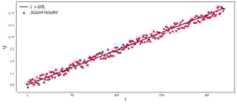
Если бы мы не знали закон Ома, то могли бы найти зависимость эмпирически, изменяя и измеряя , поддерживая при этом фиксированным. Тогда мы бы увидели, что график зависимости от дает более или менее прямую линию, проходящую через начало координат. Мы сказали «более или менее», так как, хотя зависимость фактически точная, наши измерения могут содержать малые ошибки, и поэтому точки на графике, возможно не попадут строго на линию, а будут разбросаны вокруг нее случайным образом.
График 1 «Зависимость от »
Код отрисовки графика
import matplotlib.pyplot as plt
%matplotlib inline

import numpy as np

import random

R = 13.75

x_line = np.arange(0,220,1)
y_line = []
for i in x_line:
    y_line.append(i/R)

y_dot = []
for i in y_line:
    y_dot.append(i+random.uniform(-0.9,0.9))


fig, axes = plt.subplots(figsize = (14,6), dpi = 80)
plt.plot(x_line,y_line,color = 'purple',lw = 3, label = 'I = U/R')
plt.scatter(x_line,y_dot,color = 'red', label = 'Actual results')
plt.xlabel('I', size = 16)
plt.ylabel('U', size = 16)
plt.legend(prop = {'size': 14})
plt.show()
02. Необходимость преобразований уравнения линейной регрессии
Рассмотрим очередной пример. Представим, что мы работаем в банке и перед нами задача определить вероятность возврата кредита заемщиком в зависимости от некоторых факторов. Для упрощения задачи, рассмотрим только два фактора: месячная зарплата заемщика и месячный размер платежа на погашение кредита.
Задача очень условная, но на этом примере мы сможем понять, почему для ее решения недостаточно применения функции линейной регрессии, а также узнаем какие преобразования с функцией требуется провести.
Возвращаемся к примеру. Понятно, что чем выше зарплата, тем больше заемщик сможет ежемесячно направлять на погашение кредита. При этом, для определенного диапазона зарплат эта зависимость будет вполне себе линейная. Например, возьмем диапазон зарплат от 60.000Р до 200.000Р и предположим, что в указанном диапазоне заработных плат, зависимость размера ежемесячного платежа от размера заработной платы — линейная. Допустим, для указанного диапазона размера заработных плат было выявлено, что соотношение зарплаты к платежу не может опускаться ниже 3 и еще у заемщика должно оставаться в запасе 5.000Р. И только в таком случае, мы будем считать, что заемщик вернет кредит банку. Тогда, уравнение линейной регрессии примет вид:

где  ,
,  ,
,  ,
,  — зарплата
  -го заемщика,
  — платеж по кредиту -го заемщика.
Подставляя в уравнение зарплату и платеж по кредиту с фиксированными параметрами можно принять решение о выдаче или отказе кредита.
Забегая вперед, отметим, что, при заданных параметрах функция линейной регрессии, применяемая в функции логистичиеского отклика будет выдавать большие значения, которые затруднят проведение расчетов по определению вероятностей погашения кредита. Поэтому, предлагается уменьшить наши коэффициенты, скажем так, в 25.000 раз. От этого преобразования в коэффициентах, решение о выдачи кредита не изменится. Запомним этот момент на будущее, а сейчас чтобы было еще понятнее, о чем речь, рассмотрим ситуация с тремя потенциальными заемщиками.
Таблица 1 «Потенциальные заемщики»

Код для формирования таблицы
import pandas as pd

r = 25000.0
w_0 = -5000.0/r
w_1 = 1.0/r
w_2 = -3.0/r

data = {'The borrower':np.array(['Vasya', 'Fedya', 'Lesha']),
        'Salary':np.array([120000,180000,210000]),
       'Payment':np.array([3000,50000,70000])}

df = pd.DataFrame(data)

df['f(w,x)'] = w_0 + df['Salary']*w_1 + df['Payment']*w_2

decision = []
for i in df['f(w,x)']:
    if i > 0:
        dec = 'Approved'
        decision.append(dec)
    else:
        dec = 'Refusal'
        decision.append(dec)

df['Decision'] = decision

df[['The borrower', 'Salary', 'Payment', 'f(w,x)', 'Decision']]
В соответствии с данными таблицы, Вася при зарплате в 120.000Р хочет получить такой кредит, чтобы ежемесячного гасить его по 3.000Р. Нами было определено, что для одобрения кредита, размер заработной платы Васи должен превышать в три раза размер платежа, и чтобы еще оставалось 5.000Р. Этому требованию Вася удовлетворяет:  . Остается даже 106.000Р. Несмотря на то, что при расчете
  мы уменьшили коэффициенты в 25.000 раз, результат получили тот же — кредит может быть одобрен. Федя тоже получит кредит, а вот Леше, несмотря на то, что он получает больше всех, придется поумерить свои аппетиты.
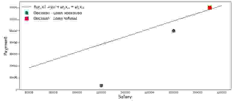
Нарисуем график по такому случаю.
График 2 «Классификация заемщиков»
Код для отрисовки графика
salary = np.arange(60000,240000,20000)
payment = (-w_0-w_1*salary)/w_2


fig, axes = plt.subplots(figsize = (14,6), dpi = 80)
plt.plot(salary, payment, color = 'grey', lw = 2, label = '$f(w,x_i)=w_0 + w_1x_{i1} + w_2x_{i2}$')
plt.plot(df[df['Decision'] == 'Approved']['Salary'], df[df['Decision'] == 'Approved']['Payment'],
         'o', color ='green', markersize = 12, label = 'Decision - Loan approved')
plt.plot(df[df['Decision'] == 'Refusal']['Salary'], df[df['Decision'] == 'Refusal']['Payment'],
         's', color = 'red', markersize = 12, label = 'Decision - Loan refusal')
plt.xlabel('Salary', size = 16)
plt.ylabel('Payment', size = 16)
plt.legend(prop = {'size': 14})
plt.show()
Итак, наша прямая, построенная в соответствии с функцией  , отделяет «плохих» заемщиков от «хороших». Те заемщики, у кого желания не совпадают с возможностями находятся выше прямой (Леша), те же, кто способен согласно параметрам нашей модели, вернуть кредит, находятся под прямой (Вася и Федя). Иначе можно сказать так — наша прямая разделяет заемщиков на два класса. Обозначим их следующим образом: к классу
  отнесем тех заемщиков, которые скорее всего вернут кредит, к классу
  или
или  отнесем тех заемщиков, которые скорее всего не смогут вернуть кредит.
Обобщим выводы из этого простенького примера. Возьмем точку  и, подставляя координаты точки в соответствующее уравнение прямой , рассмотрим три варианта:
- Если точка находится под прямой, и мы относим ее к классу , то значение функции будет положительным от до . Значит мы можем считать, что вероятность погашения кредита, находится в пределах . Чем больше значение функции, тем выше вероятность.
- Если точка находится над прямой и мы относим ее к классу или , то значение функции будет отрицательным от до . Тогда мы будем считать, что вероятность погашения задолженности находится в пределах и, чем больше по модулю значение функции, тем выше наша уверенность.
- Точка находится на прямой, на границе между двумя классами. В таком случае значение функции будет равно и вероятность погашения кредита равна .
![$(0.5,1]$](https://habrastorage.org/getpro/habr/formulas/e52/d01/8f8/e52d018f87e1844bc2e714af79f0cdf0.svg) . Чем больше значение функции, тем выше вероятность.
. Чем больше значение функции, тем выше вероятность. и, чем больше по модулю значение функции, тем выше наша уверенность.
 .
.
Теперь, представим, что у нас не два фактора, а десятки, заемщиков не три, а тысячи. Тогда вместо прямой у нас будет m-мерная плоскость и коэффициенты  у нас будут взяты не с потолка, а выведены по всем правилам, да на основе накопленных данных о заемщиках, вернувших или не вернувших кредит. И действительно, заметьте, мы сейчас отбираем заемщиков при уже известных коэффициентах . На самом же деле, задача модели логистической регрессии как раз и состоит в том, чтобы определить параметры , при которых значение функции потерь Logistic Loss будет стремиться к минимальному. Но о том, как рассчитывается вектор , мы еще узнаем в 5-м разделе статьи. А пока возвращаемся на землю обетованную — к нашему банкиру и трем его клиентам.
Благодаря функции мы знаем кому можно дать кредит, а кому нужно отказать. Но с такой информацией к директору идти нельзя, ведь от нас хотели получить вероятность возврата кредита каждым заемщиком. Что делать? Ответ простой — нам нужно как-то преобразовать функцию , значения которой лежат в диапазоне  на функцию, значения которой будут лежать в диапазоне
 ![$[0,1]$](https://habrastorage.org/getpro/habr/formulas/a5d/538/f83/a5d538f83bd73f9d1c9e8338db9a398a.svg) . И такая функция существует, ее называют функцией логистического отклика или обратного-логит преобразования. Знакомьтесь:
. И такая функция существует, ее называют функцией логистического отклика или обратного-логит преобразования. Знакомьтесь:

Посмотрим по шагам как получается функция логистического отклика. Отметим, что шагать мы будем в обратную сторону, т.е. мы предположим, что нам известно значение вероятности, которое лежит в пределах от до  и далее мы будем «раскручивать» это значение на всю область чисел от
  до
до  .
.
03. Выводим функцию логистического отклика
Шаг 1. Переведем значения вероятности в диапазон

На время трансформации функции в функцию логистического отклика  мы оставим в покое нашего кредитного аналитика, а вместо этого пройдемся по букмекерским конторам. Нет, конечно, ставки делать мы не будем, все что нас там интересует, так это смысл выражения, например, шанс 4 к 1. Шансы, знакомые всем делающим ставки игрокам, являются соотношением «успехов» к «неуспехам». С точки зрения вероятностей, шансы — это вероятность наступления события, деленная на вероятность того, что событие не произойдет. Запишем формулу шанса наступления события
  :
:

, где  — вероятность наступления события,
  — вероятность НЕ наступления события
Например, если вероятность того, что молодой, сильный и резвый конь по прозвищу «Ветерок» обойдет на скачках старую и дряблую старушку по кличке «Матильда» равняется  , то шансы на успех «Ветерка» составят
  к
к  и наоборот, зная шансы, нам не составит труда вычислить вероятность :

Таким образом, мы научились «переводить» вероятность в шансы, которые принимают значения от до . Сделаем еще один шаг и научимся «переводить» вероятность на всю числовую прямую от до .
Шаг 2. Переведем значения вероятности в диапазон
Шаг этот очень простой — прологарифмируем шансы по основанию числа Эйлера  и получим:

Теперь мы знаем, что если  , то вычислить значение будет очень просто и, более того, оно должно быть положительным:
  . Так и есть.
Ради любопытства проверим, что если  , тогда мы ожидаем увидеть отрицательное значение . Проверяем:
  . Все верно.
Теперь мы знаем как перевести значение вероятности от до на всю числовую прямую от до . В следующем шаге сделаем все наоборот.
А пока, отметим, что в соответствии с правилами логарифмирования, зная значение функции , можно вычислить шансы:

Этот способ определения шансов нам пригодится на следующем шаге.
Шаг 3. Выведем формулу для определения
Итак, мы научились, зная , находить значения функции . Однако, на самом деле нам нужно все с точностью до наоборот — зная значение находить . Для этого обратимся к такому понятию как обратная функция шансов, в соответствии с которой:

В статье мы не будем выводить вышеобозначенную формулу, но проверим на цифрах из примера выше. Мы знаем, что при шансах равными 4 к 1 ( ), вероятность наступления события равна 0.8 (). Сделаем подстановку:
  . Это совпадает с нашими вычислениями, проведенными ранее. Двигаемся далее.
На прошлом шаге мы вывели, что  , а значит можно сделать замену в обратной функции шансов. Получим:

Разделим и числитель и знаменатель на  , тогда:

На всякий пожарный, дабы убедиться, что мы нигде не ошиблись, сделаем еще одну небольшую проверку. На шаге 2, мы для определили, что  . Тогда, подставив значение в функцию логистического отклика, мы ожидаем получить . Подставляем и получаем:
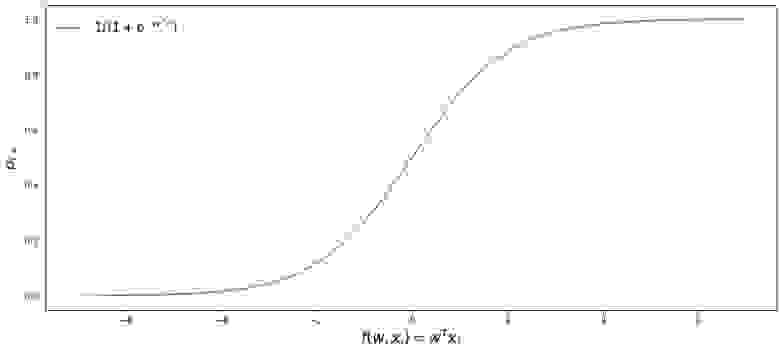
Поздравляю вас, уважаемый читатель, мы только что вывели и протестировали функцию логистического отклика. Давайте посмотрим на график функции.
График 3 «Функция логистического отклика»
Код для отрисовки графика
import math

def logit (f):
    return 1/(1+math.exp(-f))

f = np.arange(-7,7,0.05)
p = []

for i in f:
    p.append(logit(i))

fig, axes = plt.subplots(figsize = (14,6), dpi = 80)
plt.plot(f, p, color = 'grey', label = '$ 1 / (1+e^{-w^Tx_i})$')
plt.xlabel('$f(w,x_i) = w^Tx_i$', size = 16)
plt.ylabel('$p_{i+}$', size = 16)
plt.legend(prop = {'size': 14})
plt.show()
В литературе также можно встретить название данной функции как сигмоид-функция. По графику хорошо заметно, что основное изменение вероятности принадлежности объекта к классу происходит на относительно небольшом диапазоне , где-то от  до
до  .
.
Предлагаю вернуться к нашему кредитному аналитику и помочь ему с вычислением вероятности погашения кредитов, иначе он рискует остаться без премии
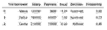
Таблица 2 «Потенциальные заемщики»
Код для формирования таблицы
proba = []
for i in df['f(w,x)']:
    proba.append(round(logit(i),2))

df['Probability'] = proba

df[['The borrower', 'Salary', 'Payment', 'f(w,x)', 'Decision', 'Probability']]
Итак, вероятность возврата кредита мы определили. В целом, это похоже на правду.
Действительно, вероятность того что Вася при зарплате в 120.000Р сможет ежемесячно отдавать в банк 3.000Р близка к 100%. Кстати, мы должны понимать, что банк может выдать кредит и Леше в том случае, если политикой банка предусмотрено, например, кредитовать клиентов с вероятностью возврата кредита более, ну скажем, 0.3. Просто в таком случае банк сформирует больший резерв под возможные потери.
Также следует отметить, что соотношение зарплаты к платежу не менее 3 и с запасом в 5.000Р было взято с потолка. Поэтому нам нельзя было использовать в первоначальном виде вектор весов  . Нам требовалось сильно уменьшить коэффициенты и в таком случае мы разделили каждый коэффициент на 25.000, то есть по сути мы подогнали результат. Но это сделано было специально, чтобы упростить понимание материала на начальном этапе. В жизни, же нам потребуется не выдумывать и подгонять коэффициенты, а находить их. Как раз в следующих разделах статьи мы выведем уравнения, с помощью которых подбираются параметры .
04. Метод наименьших квадратов при определении вектора весов в функции логистического отклика
Нам уже известен такой метод подбора вектора весов , как метод наименьших квадратов (МНК) и собственно, почему бы нам тогда не использовать его в задачах бинарной классификации? Действительно, ничто не мешает использовать МНК, только вот данный способ в задачах классификации дает результаты менее точные, нежели Logistic Loss. Этому есть теоретическое обоснование. Давайте для начала посмотрим на один простой пример.
Предположим, что наши модели (использующие MSE и Logistic Loss) уже начали подбор вектора весов и мы остановили расчет на каком-то шаге. Неважно, в середине, в конце или в начале, главное, что у нас уже есть какие-то значения вектора весов и допустим, что на этом шаге, вектора весов для обеих моделей не имеют различий. Тогда возьмем полученные веса и подставим их в функцию логистического отклика ( ) для какого-нибудь объекта, который относится к классу . Исследуем два случая, когда в соответствии с подобранным вектором весов наша модель сильно ошибается и наоборот — модель сильно уверена в том, что объект относится к классу . Посмотрим какие штрафы будут «выписаны» при использовании МНК и Logistic Loss.
Код для расчета штрафов в зависимости от используемой функции потерь
# класс объекта
y = 1
# вероятность отнесения объекта к классу в соответствии с параметрами w
proba_1 = 0.01

MSE_1 = (y - proba_1)**2
print 'Штраф MSE при грубой ошибке =', MSE_1

# напишем функцию для вычисления f(w,x) при известной вероятности отнесения объекта к классу +1 (f(w,x)=ln(odds+))
def f_w_x(proba):
    return math.log(proba/(1-proba))

LogLoss_1 = math.log(1+math.exp(-y*f_w_x(proba_1)))
print 'Штраф Log Loss при грубой ошибке =', LogLoss_1

proba_2 = 0.99

MSE_2 = (y - proba_2)**2
LogLoss_2 = math.log(1+math.exp(-y*f_w_x(proba_2)))

print '**************************************************************'
print 'Штраф MSE при сильной уверенности =', MSE_2
print 'Штраф Log Loss при сильной уверенности =', LogLoss_2
Случай с грубой ошибкой — модель относит объект к классу с вероятностью в 0,01
Штраф при использовании МНК составит:

Штраф при использовании Logistic Loss составит:

Случай с сильной уверенностью — модель относит объект к классу с вероятностью в 0,99
Штраф при использовании МНК составит:

Штраф при использовании Logistic Loss составит:

Этот пример хорошо иллюстрирует, что при грубой ошибке функция потерь Log Loss штрафует модель значительно сильнее, чем MSE. Давайте теперь разберемся, каковы теоретические предпосылки использования функции потерь Log Loss в задачах классификации.
05. Метод максимального правдоподобия и логистическая регрессия
Как и было обещано в начале, статья изобилует простыми примерами. В студии очередной пример и старые гости — заемщики банка: Вася, Федя и Леша.
На всякий пожарный, перед тем как развивать пример, напомню, что в жизни мы имеем дело с обучающей выборкой из тысяч или миллионов объектов с десятками или сотнями признаков. Однако здесь цифры взяты так, чтобы они легко укладывались в голове начинающего датасайнтеста.
Возвращаемся к примеру. Представим, что директор банка решил выдать кредит всем нуждающимся, несмотря на то, что алгоритм подсказывал не выдавать его Леше. И вот прошло достаточно времени и нам стало известно кто из трех героев погасил кредит, а кто нет. Что и следовало ожидать: Вася и Федя погасили кредит, а Леша — нет. Теперь давайте представим, что этот результат будет для нас новой обучающей выборкой и, при этом у нас как будто исчезли все данные о факторах, влияющих на вероятность погашения кредита (зарплата заемщика, размер ежемесячного платежа). Тогда интуитивно мы можем полагать, что каждый третий заемщик не возвращает банку кредит или другими словами вероятность возврата кредита следующим заемщиком  . Этому интуитивному предположению есть теоретическое подтверждение и основывается оно на методе максимального правдоподобия, часто в литературе его называют принципом максимального правдоподобия.
Для начала познакомимся с понятийным аппаратом.
Правдоподобие выборки — это вероятность получения именно такой выборки, получения именно таких наблюдений / результатов, т.е. произведение вероятностей получения каждого из результатов выборки (например, погашен или не погашен кредит Васей, Федей и Лешей одновременно).
Функция правдоподобия связывает правдоподобие выборки со значениями параметров распределения.
В нашем случае, обучающая выборка представляет собой обобщённую схему Бернулли, в которой случайная величина принимает всего два значения: или . Следовательно, правдоподобие выборки можно записать как функцию правдоподобия от параметра  следующим образом:


Вышеуказанную запись можно интерпретировать так. Совместная вероятность того, что Вася и Федя погасят кредит равна  , вероятность того что Леша НЕ погасит кредит равна
  (так как имело место именно НЕ погашение кредита), следовательно совместная вероятность всех трех событий равна
  .
.
Метод максимального правдоподобия — это метод оценки неизвестного параметра путём максимизации функции правдоподобия. В нашем случае требуется найти такое значение , при котором  достигает максимума.
Откуда собственно идея – искать значение неизвестного параметра, при котором функция правдоподобия достигает максимума? Истоки идеи проистекают из представления о том, что выборка – это единственный, доступный нам, источник знания о генеральной совокупности. Все, что нам известно о генеральной совокупности, представлено в выборке. Поэтому, все, что мы можем сказать, так это то, что выборка – это наиболее точное отражение генеральной совокупности, доступное нам. Следовательно, нам требуется найти такой параметр, при котором имеющаяся выборка становится наиболее вероятной.
Очевидно, мы имеем дело с оптимизационной задачей, в которой требуется найти точку экстремума функции. Для нахождения точки экстремума необходимо рассмотреть условие первого порядка, то есть приравнять производную функции к нулю и решить уравнение относительно искомого параметра. Однако поиски производной произведения большого количества множителей могут оказаться делом затяжным, чтобы этого избежать существует специальный прием — переход к логарифму функции правдоподобия. Почему возможен такой переход? Обратим внимание на то, что мы ищем не сам экстремум функции , а точку экстремума, то есть то значение неизвестного параметра , при котором достигает максимума. При переходе к логарифму точка экстремума не меняется (хотя сам экстремум будет отличаться), так как логарифм — монотонная функция.
Давайте, в соответствии с вышеизложенным, продолжим развивать наш пример с кредитами у Васи, Феди и Леши. Для начала перейдем к логарифму функции правдоподобия:

Теперь мы можем с легкостью продифференцировать выражение по :

И наконец, рассмотрим условие первого порядка — приравняем производную функции к нулю:

Таким образом, наша интуитивная оценка вероятности погашения кредита была теоретически обоснована.
Отлично, но что нам теперь делать с такой информацией? Если мы будем считать, что каждый третий заемщик не вернет банку деньги, то последний неизбежно разорится. Так-то оно так, да только при оценке вероятности погашения кредита равной  мы не учли факторы, влияющие на возврат кредита: заработная плата заемщика и размер ежемесячного платежа. Вспомним, что ранее мы рассчитали вероятность возврата кредита каждым клиентом с учетом этих самых факторов. Логично, что и вероятности у нас получились отличные от константы равной .
Давайте определим правдоподобие выборок:
Код для расчетов правдоподобий выборок
from functools import reduce

def likelihood(y,p):
    line_true_proba = []
    for i in range(len(y)):
        ltp_i = p[i]**y[i]*(1-p[i])**(1-y[i])
        line_true_proba.append(ltp_i)
    likelihood = []
    return reduce(lambda a, b: a*b, line_true_proba)


y = [1.0,1.0,0.0]
p_log_response = df['Probability']
const = 2.0/3.0
p_const = [const, const, const]


print 'Правдоподобие выборки при константном значении p=2/3:', round(likelihood(y,p_const),3)

print '****************************************************************************************************'

print 'Правдоподобие выборки при расчетном значении p:', round(likelihood(y,p_log_response),3)
Правдоподобие выборки при константном значении :

Правдоподобие выборки при расчете вероятности погашения кредита с учетом факторов  :
:


Правдоподобие выборки с вероятностью, посчитанной в зависимости от факторов оказалось выше правдоподобия при константном значении вероятности. О чем это говорит? Это говорит о том, что знания о факторах позволили подобрать более точно вероятность погашения кредита для каждого клиента. Поэтому, при выдаче очередного кредита, правильнее будет использовать, предложенную в конце 3-го раздела статьи, модель оценки вероятности погашения задолженности.
Но тогда, если нам требуется максимизировать функцию правдоподобия выборки, то почему бы не использовать какой-нибудь алгоритм, который будет выдавать вероятности для Васи, Феди и Леши, например, равными 0.99, 0.99 и 0.01 соответственно. Возможно такой алгоритм и хорошо себя проявит на обучающей выборке, так как приблизит значение правдоподобия выборки к , но, во-первых, у такого алгоритма будут, скорее всего трудности с обобщающей способностью, во-вторых, этот алгоритм будет точно не линейным. И если, методы борьбы с переобучением (равно слабая обобщающая способность) явно не входят в план этой статьи, то по второму пункту давайте пройдемся подробнее. Для этого, достаточно ответить на простой вопрос. Может ли вероятность погашения кредита Васей и Федей быть одинаковой с учетом известных нам факторов? С точки зрения здравой логики конечно же нет, не может. Так на погашение кредита Вася будет отдавать 2.5% своей зарплаты в месяц, а Федя — почти 27,8%. Также на графике 2 «Классификация клиентов» мы видим, что Вася находится значительно дальше от линии, разделяющей классы, чем Федя. Ну и наконец, мы знаем, что функция  для Васи и Феди принимает различные значения: 4.24 для Васи и 1.0 для Феди. Вот если бы Федя, например, зарабатывал на порядок больше или кредит поменьше просил, то тогда вероятности погашения кредита у Васи и Феди были бы схожими. Другими словами, линейную зависимость не обманешь. И если бы мы действительно рассчитали коэффициенты , а не взяли их с потолка, то могли бы смело заявить, что наши значения лучше всего позволяют оценить вероятность погашения кредита каждым заемщиком, но так как мы условились считать, что определение коэффициентов было проведено по всем правилам, то мы так и будем считать — наши коэффициенты позволяют дать лучшую оценку вероятности
Однако мы отвлеклись. В этом разделе нам надо разобраться как определяется вектор весов , который необходим для оценки вероятности возврата кредита каждым заемщиком.
Кратко резюмируем, с каким арсеналом мы выступаем на поиски коэффициентов :
1. Мы предполагаем, что зависимость между целевой переменной (прогнозным значением) и фактором, оказывающим влияние на результат — линейная. По этой причине применяется функция линейной регрессии вида  , линия которого делит объекты (клиентов) на классы и или (клиенты, способные погасить кредит и не способные). В нашем случае уравнение имеет вид .
2. Мы используем функцию обратного логит-преобразования вида для определения вероятности принадлежности объекта к классу .
3. Мы рассматриваем нашу обучающую выборку как реализацию обобщенной схемы Бернулли, то есть для каждого объекта генерируется случайная величина, которая с вероятностью (своей для каждого объекта) принимает значение 1 и с вероятностью  – 0.
– 0.
4. Мы знаем, что нам требуется максимизировать функцию правдоподобия выборки с учетом принятых факторов для того, чтобы имеющаяся выборка стала наиболее правдоподобной. Другими словами, нам нужно подобрать такие параметры, при которых выборка будет наиболее правдоподобной. В нашем случае подбираемый параметр — это вероятность погашения кредита , которая в свою очередь зависит от неизвестных коэффициентов . Значит нам требуется найти такой вектор весов , при котором правдоподобие выборки будет максимальным.
5. Мы знаем, что для максимизации функции правдоподобия выборки можно использовать метод максимального правдоподобия. И мы знаем все хитрые приемы для работы с этим методом.
Вот такая многоходовочка получается
А теперь вспомним, что в самом начале статьи мы хотели вывести два вида функции потерь Logistic Loss в зависимости от того как обозначаются классы объектов. Так повелось, что в задачах классификации с двумя классами, классы обозначают как и или . В зависимости от обозначения, на выходе будет соответствующая функция потерь.
Случай 1. Классификация объектов на и
Раннее, при определении правдоподобия выборки, в котором вероятность погашения задолженности заемщиком рассчитывалась исходя из факторов и заданных коэффициентов , мы применили формулу:

На самом деле  — это значение функции логистического отклика при заданном векторе весов
Тогда нам ничто не мешает записать функцию правдоподобия выборки так:

Бывает так, что иногда, некоторым начинающим аналитикам сложно сходу понять, как эта функция работает. Давайте рассмотрим 4 коротких примера, которые все прояснят:
1. Если  (т.е. в соответствии с обучающей выборкой объект относится к классу +1), а наш алгоритм
  определяет вероятность отнесения объекта к классу равной 0.9, то вот этот кусочек правдоподобия выборки будет рассчитываться так:

2. Если , а  , то расчет будет таким:

3. Если  , а , то расчет будет таким:

4. Если , а  , то расчет будет таким:

Очевидно, что функция правдоподобия будет максимизироваться в случаях 1 и 3 или в общем случае — при правильно отгаданных значениях вероятностей отнесения объекта к классу .
В связи с тем, что при определении вероятности отнесения объекта к классу нам не известны только коэффициенты , то мы их и будем искать. Как и говорилось выше, это задача оптимизации, в которой для начала нам требуется найти производную от функции правдоподобия по вектору весов . Однако предварительно имеет смысл упростить себе задачу: производную будем искать от логарифма функции правдоподобия.

Почему после логарифмирования, в функции логистической ошибки, мы поменяли знак с  на
на  . Все просто, так как в задачах оценки качества модели принято минимизировать значение функции, то мы умножили правую часть выражения на и соответственно вместо максимизации, теперь минимизируем функцию.
Собственно, сейчас, на ваших глазах была много страдальчески выведена функция потерь — Logistic Loss для обучающей выборки с двумя классами: и .
Теперь, для нахождения коэффициентов, нам потребуется всего лишь найти производную функции логистической ошибки и далее, используя численные методы оптимизации, такие как градиентный спуск или стохастический градиентный спуск, подобрать наиболее оптимальные коэффициенты . Но, учитывая, уже не малый объем статьи, предлагается провести дифференцирование самостоятельно или, быть может, это будет темой для следующей статьи с большим количеством арифметики без столь подробных примеров.
Случай 2. Классификация объектов на и
Подход здесь будет такой же, как и с классами и , но сама дорожка к выводу функции потерь Logistic Loss, будет более витиеватой. Приступаем. Будем для функции правдоподобия использовать оператор «если…, то…». То есть, если -ый объект относится к классу , то для расчета правдоподобия выборки используем вероятность , если объект относится к классу , то в правдоподобие подставляем  . Вот так выглядит функция правдоподобия:
![$P(\mkern 5mu \vec{y} \mkern 5mu |\mkern 5mu \sigma(\vec{w}^TX)) \mkern 5mu = \mkern 5mu \prod\limits_{i=1}^n \sigma(\vec{w}^T\vec{x_i})^{[y_i=+1]} \mkern 10mu (1-\sigma(\vec{w}^T\vec{x_i})^{[y_i=-1])} \mkern 10mu \rightarrow \mkern 10mu max$](https://habrastorage.org/getpro/habr/formulas/4a1/375/d87/4a1375d876abb71c1dd376a63d13c727.svg)
На пальцах распишем как это работает. Рассмотрим 4 случая:
1. Если и  , то в правдоподобие выборки «пойдет»
2. Если и  , то в правдоподобие выборки «пойдет»
3. Если  и , то в правдоподобие выборки «пойдет»
4. Если и , то в правдоподобие выборки «пойдет» 
Очевидно, что в 1 и 3 случае, когда вероятности были правильно определены алгоритмом, функция правдоподобия будет максимизироваться, то есть именно это мы и хотели получить. Однако, такой подход достаточно громоздок и далее мы рассмотрим более компактную запись. Но для начала, логарифмируем функцию правдоподобия с заменой знака, так как теперь мы будем минимизировать ее.
![$L_{log}(X,\vec{y},\vec{w}) = \sum\limits_{i=1}^n(-[y_i=+1] \mkern 2mu log_e \mkern 5mu \sigma(\vec{w}^T \vec{x_i}) - [y_i=-1] \mkern 2mu log_e \mkern 5mu (1 - \sigma(\vec{w}^T \vec{x_i})) ) \rightarrow min$](https://habrastorage.org/getpro/habr/formulas/130/e8f/691/130e8f691883e01464d6cff33b3855b8.svg)
Подставим вместо  выражение
  :
:
![$L_{log}(X,\vec{y},\vec{w}) = \sum\limits_{i=1}^n(-[y_i=+1] \mkern 2mu log_e \mkern 5mu (\frac{1}{1+e^{-\vec{w}^T\vec{x_i}}}) - [y_i=-1] \mkern 2mu log_e \mkern 5mu (1 - \frac{1}{1+e^{-\vec{w}^T\vec{x_i}}})) \rightarrow min$](https://habrastorage.org/getpro/habr/formulas/c2c/0ab/36e/c2c0ab36e7845ed6bc08f3bfa7f7a6f5.svg)
Упростим правое слагаемое под логарифмом, используя простые арифметические приемы и получим:
![$L_{log}(X,\vec{y},\vec{w}) = \sum\limits_{i=1}^n(-[y_i=+1] \mkern 2mu log_e \mkern 5mu (\frac{1}{1+e^{-\vec{w}^T\vec{x_i}}}) - [y_i=-1] \mkern 2mu log_e \mkern 5mu (\frac{1}{1+e^{\vec{w}^T\vec{x_i}}})) \rightarrow min$](https://habrastorage.org/getpro/habr/formulas/c5e/32f/f29/c5e32ff297d5114261c85aa8b00d74e4.svg)
А теперь настало время избавиться от оператора «если…, то…». Заметим, что когда объект  относится к классу , то в выражении под логарифмом, в знаменателе, возводится в степень
  , если объект относится к классу , то $e$ возводится в степень
  . Следовательно запись степени можно упростить — объединить оба случая в один:
  . Тогда функция логистической ошибки примет вид:

В соответствии с правилами логарифмирования, перевернем дробь и вынесем знак «» (минус) за логарифм, получим:

Перед вами функция потерь logistic Loss, которая применяется в обучающей выборке с объектами относимых к классам: и .
Что ж, на этом моменте я откланиваюсь и мы завершаем статью.
 Предыдущая работа автора — «Приводим уравнение линейной регрессии в матричный вид»
Вспомогательные материалы
1. Литература
1) Прикладной регрессионный анализ / Н. Дрейпер, Г. Смит – 2-е изд. – М.: Финансы и статистика, 1986 (перевод с английского)
2) Теория вероятностей и математическая статистика / В.Е. Гмурман — 9-е изд. — М.: Высшая школа, 2003
3) Теория вероятностей / Н.И. Чернова — Новосибирск: Новосибирский государственный университет, 2007
4) Бизнес-аналитика: от данных к знаниям / Паклин Н. Б., Орешков В. И. — 2-е изд. — Санкт-Петербург: Питер, 2013
5) Data Science Наука о данных с нуля / Джоэл Грас — Санкт-Петербург: БХВ Петербург, 2017
6) Практическая статистика для специалистов Data Science / П.Брюс, Э.Брюс — Санкт-Петербург: БХВ Петербург, 2018
2. Лекции, курсы (видео)
1) Суть метода максимального правдоподобия, Борис Демешев
2) Метод максимального правдоподобия в непрерывном случае, Борис Демешев
3) Логистическая регрессия. Открытый курс ODS, Yury Kashnitsky
4) Лекция 4, Евгений Соколов (с 47 минуты видео)
5) Логистическая регрессия, Вячеслав Воронцов
3. Интернет-источники
1) Линейные модели классификации и регрессии
2) Как легко понять логистическую регрессию
3) Логистическая функция ошибки
4) Независимые испытания и формула Бернули
5) Баллада о ММП
6) Метод максимального правдоподобия
7) Формулы и свойства логарифмов
 Почему число ?
9) Линейный классификатор
9) Jupyter notebook на гитхабе
«Logit model» redirects here. Not to be confused with Logit function.
In statistics, the logistic model (or logit model) is a statistical model that models the probability of an event taking place by having the log-odds for the event be a linear combination of one or more independent variables. In regression analysis, logistic regression[1] (or logit regression) is estimating the parameters of a logistic model (the coefficients in the linear combination). Formally, in binary logistic regression there is a single binary dependent variable, coded by an indicator variable, where the two values are labeled «0» and «1», while the independent variables can each be a binary variable (two classes, coded by an indicator variable) or a continuous variable (any real value). The corresponding probability of the value labeled «1» can vary between 0 (certainly the value «0») and 1 (certainly the value «1»), hence the labeling;[2] the function that converts log-odds to probability is the logistic function, hence the name. The unit of measurement for the log-odds scale is called a logit, from logistic unit, hence the alternative names. See § Background and § Definition for formal mathematics, and § Example for a worked example.
Binary variables are widely used in statistics to model the probability of a certain class or event taking place, such as the probability of a team winning, of a patient being healthy, etc. (see § Applications), and the logistic model has been the most commonly used model for binary regression since about 1970.[3] Binary variables can be generalized to categorical variables when there are more than two possible values (e.g. whether an image is of a cat, dog, lion, etc.), and the binary logistic regression generalized to multinomial logistic regression. If the multiple categories are ordered, one can use the ordinal logistic regression (for example the proportional odds ordinal logistic model[4]). See § Extensions for further extensions. The logistic regression model itself simply models probability of output in terms of input and does not perform statistical classification (it is not a classifier), though it can be used to make a classifier, for instance by choosing a cutoff value and classifying inputs with probability greater than the cutoff as one class, below the cutoff as the other; this is a common way to make a binary classifier.
Analogous linear models for binary variables with a different sigmoid function instead of the logistic function (to convert the linear combination to a probability) can also be used, most notably the probit model; see § Alternatives. The defining characteristic of the logistic model is that increasing one of the independent variables multiplicatively scales the odds of the given outcome at a constant rate, with each independent variable having its own parameter; for a binary dependent variable this generalizes the odds ratio. More abstractly, the logistic function is the natural parameter for the Bernoulli distribution, and in this sense is the «simplest» way to convert a real number to a probability. In particular, it maximizes entropy (minimizes added information), and in this sense makes the fewest assumptions of the data being modeled; see § Maximum entropy.
The parameters of a logistic regression are most commonly estimated by maximum-likelihood estimation (MLE). This does not have a closed-form expression, unlike linear least squares; see § Model fitting. Logistic regression by MLE plays a similarly basic role for binary or categorical responses as linear regression by ordinary least squares (OLS) plays for scalar responses: it is a simple, well-analyzed baseline model; see § Comparison with linear regression for discussion. The logistic regression as a general statistical model was originally developed and popularized primarily by Joseph Berkson,[5] beginning in Berkson (1944), where he coined «logit»; see § History.
Applications[edit]
Logistic regression is used in various fields, including machine learning, most medical fields, and social sciences. For example, the Trauma and Injury Severity Score (TRISS), which is widely used to predict mortality in injured patients, was originally developed by Boyd et al. using logistic regression.[6] Many other medical scales used to assess severity of a patient have been developed using logistic regression.[7][8][9][10] Logistic regression may be used to predict the risk of developing a given disease (e.g. diabetes; coronary heart disease), based on observed characteristics of the patient (age, sex, body mass index, results of various blood tests, etc.).[11][12] Another example might be to predict whether a Nepalese voter will vote Nepali Congress or Communist Party of Nepal or Any Other Party, based on age, income, sex, race, state of residence, votes in previous elections, etc.[13] The technique can also be used in engineering, especially for predicting the probability of failure of a given process, system or product.[14][15] It is also used in marketing applications such as prediction of a customer’s propensity to purchase a product or halt a subscription, etc.[16] In economics, it can be used to predict the likelihood of a person ending up in the labor force, and a business application would be to predict the likelihood of a homeowner defaulting on a mortgage. Conditional random fields, an extension of logistic regression to sequential data, are used in natural language processing.
Example[edit]
Problem[edit]
As a simple example, we can use a logistic regression with one explanatory variable and two categories to answer the following question:
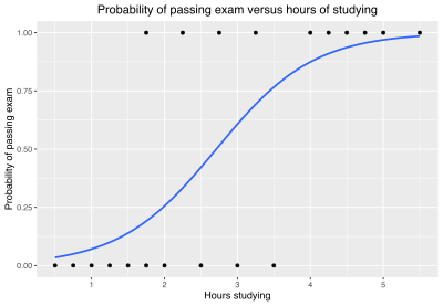
A group of 20 students spends between 0 and 6 hours studying for an exam. How does the number of hours spent studying affect the probability of the student passing the exam?
The reason for using logistic regression for this problem is that the values of the dependent variable, pass and fail, while represented by «1» and «0», are not cardinal numbers. If the problem was changed so that pass/fail was replaced with the grade 0–100 (cardinal numbers), then simple regression analysis could be used.
The table shows the number of hours each student spent studying, and whether they passed (1) or failed (0).
| Hours (xk) | 0.50 | 0.75 | 1.00 | 1.25 | 1.50 | 1.75 | 1.75 | 2.00 | 2.25 | 2.50 | 2.75 | 3.00 | 3.25 | 3.50 | 4.00 | 4.25 | 4.50 | 4.75 | 5.00 | 5.50 |
|---|---|---|---|---|---|---|---|---|---|---|---|---|---|---|---|---|---|---|---|---|
| Pass (yk) | 0 | 0 | 0 | 0 | 0 | 0 | 1 | 0 | 1 | 0 | 1 | 0 | 1 | 0 | 1 | 1 | 1 | 1 | 1 | 1 |
We wish to fit a logistic function to the data consisting of the hours studied (xk) and the outcome of the test (yk =1 for pass, 0 for fail). The data points are indexed by the subscript k which runs from  to
to  . The x variable is called the «explanatory variable», and the y variable is called the «categorical variable» consisting of two categories: «pass» or «fail» corresponding to the categorical values 1 and 0 respectively.
Model[edit]
The logistic function is of the form:

where μ is a location parameter (the midpoint of the curve, where  ) and s is a scale parameter. This expression may be rewritten as:

where  and is known as the intercept (it is the vertical intercept or y-intercept of the line
  ), and
  (inverse scale parameter or rate parameter): these are the y-intercept and slope of the log-odds as a function of x. Conversely,
  and
and  .
.
Fit[edit]
The usual measure of goodness of fit for a logistic regression uses logistic loss (or log loss), the negative log-likelihood. For a given xk and yk, write  . The
. The  are the probabilities that the corresponding
  will be unity and
  are the probabilities that they will be zero (see Bernoulli distribution). We wish to find the values of
  and
and  which give the «best fit» to the data. In the case of linear regression, the sum of the squared deviations of the fit from the data points (yk), the squared error loss, is taken as a measure of the goodness of fit, and the best fit is obtained when that function is minimized.
The log loss for the k-th point is:

The log loss can be interpreted as the «surprisal» of the actual outcome relative to the prediction , and is a measure of information content. Note that log loss is always greater than or equal to 0, equals 0 only in case of a perfect prediction (i.e., when  and
and  , or
, or  and
and  ), and approaches infinity as the prediction gets worse (i.e., when and
  or and
  ), meaning the actual outcome is «more surprising». Since the value of the logistic function is always strictly between zero and one, the log loss is always greater than zero and less than infinity. Note that unlike in a linear regression, where the model can have zero loss at a point by passing through a data point (and zero loss overall if all points are on a line), in a logistic regression it is not possible to have zero loss at any points, since is either 0 or 1, but
  .
.
These can be combined into a single expression:

This expression is more formally known as the cross-entropy of the predicted distribution  from the actual distribution
  , as probability distributions on the two-element space of (pass, fail).
The sum of these, the total loss, is the overall negative log-likelihood  , and the best fit is obtained for those choices of and for which is minimized.
Alternatively, instead of minimizing the loss, one can maximize its inverse, the (positive) log-likelihood:

or equivalently maximize the likelihood function itself, which is the probability that the given data set is produced by a particular logistic function:

This method is known as maximum likelihood estimation.
Parameter estimation[edit]
Since ℓ is nonlinear in and , determining their optimum values will require numerical methods. Note that one method of maximizing ℓ is to require the derivatives of ℓ with respect to and to be zero:


and the maximization procedure can be accomplished by solving the above two equations for and , which, again, will generally require the use of numerical methods.
The values of and which maximize ℓ and L using the above data are found to be:


which yields a value for μ and s of:


Predictions[edit]
The and coefficients may be entered into the logistic regression equation to estimate the probability of passing the exam.
For example, for a student who studies 2 hours, entering the value  into the equation gives the estimated probability of passing the exam of 0.25:


Similarly, for a student who studies 4 hours, the estimated probability of passing the exam is 0.87:


This table shows the estimated probability of passing the exam for several values of hours studying.
| Hours of study (x) |
Passing exam | ||
|---|---|---|---|
| Log-odds (t) | Odds (et) | Probability (p) | |
| 1 | −2.57 | 0.076 ≈ 1:13.1 | 0.07 |
| 2 | −1.07 | 0.34 ≈ 1:2.91 | 0.26 |
 |
0 | 1 |  = 0.50 = 0.50
|
| 3 | 0.44 | 1.55 | 0.61 |
| 4 | 1.94 | 6.96 | 0.87 |
| 5 | 3.45 | 31.4 | 0.97 |
Model evaluation[edit]
The logistic regression analysis gives the following output.
| Coefficient | Std. Error | z-value | p-value (Wald) | |
|---|---|---|---|---|
| Intercept (β0) | −4.1 | 1.8 | −2.3 | 0.021 |
| Hours (β1) | 1.5 | 0.6 | 2.4 | 0.017 |
By the Wald test, the output indicates that hours studying is significantly associated with the probability of passing the exam ( ). Rather than the Wald method, the recommended method[citation needed] to calculate the p-value for logistic regression is the likelihood-ratio test (LRT), which for these data give
  (see § Deviance and likelihood ratio tests below).
Generalizations[edit]
This simple model is an example of binary logistic regression, and has one explanatory variable and a binary categorical variable which can assume one of two categorical values. Multinomial logistic regression is the generalization of binary logistic regression to include any number of explanatory variables and any number of categories.
Background[edit]
 ; note that
  for all
  .
.
Definition of the logistic function[edit]
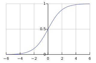
An explanation of logistic regression can begin with an explanation of the standard logistic function. The logistic function is a sigmoid function, which takes any real input , and outputs a value between zero and one.[2] For the logit, this is interpreted as taking input log-odds and having output probability. The standard logistic function  is defined as follows:

A graph of the logistic function on the t-interval (−6,6) is shown in Figure 1.
Let us assume that is a linear function of a single explanatory variable  (the case where is a linear combination of multiple explanatory variables is treated similarly). We can then express as follows:

And the general logistic function  can now be written as:

In the logistic model,  is interpreted as the probability of the dependent variable
  equaling a success/case rather than a failure/non-case. It is clear that the response variables
  are not identically distributed:
  differs from one data point
  to another, though they are independent given design matrix
  and shared parameters
  .[11]
.[11]
Definition of the inverse of the logistic function[edit]
We can now define the logit (log odds) function as the inverse  of the standard logistic function. It is easy to see that it satisfies:

and equivalently, after exponentiating both sides we have the odds:

Interpretation of these terms[edit]
In the above equations, the terms are as follows:
Definition of the odds[edit]
The odds of the dependent variable equaling a case (given some linear combination of the predictors) is equivalent to the exponential function of the linear regression expression. This illustrates how the logit serves as a link function between the probability and the linear regression expression. Given that the logit ranges between negative and positive infinity, it provides an adequate criterion upon which to conduct linear regression and the logit is easily converted back into the odds.[2]
So we define odds of the dependent variable equaling a case (given some linear combination of the predictors) as follows:

The odds ratio[edit]
For a continuous independent variable the odds ratio can be defined as:

The image represents an outline of what an odds ratio looks like in writing, through a template in addition to the test score example in the «Example» section of the contents. In simple terms, if we hypothetically get an odds ratio of 2 to 1, we can say… «For every one-unit increase in hours studied, the odds of passing (group 1) or failing (group 0) are (expectedly) 2 to 1 (Denis, 2019).
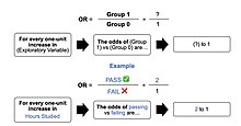

This exponential relationship provides an interpretation for : The odds multiply by  for every 1-unit increase in x.[17]
For a binary independent variable the odds ratio is defined as  where a, b, c and d are cells in a 2×2 contingency table.[18]
Multiple explanatory variables[edit]
If there are multiple explanatory variables, the above expression  can be revised to
  . Then when this is used in the equation relating the log odds of a success to the values of the predictors, the linear regression will be a multiple regression with m explanators; the parameters
  for all
  are all estimated.
Again, the more traditional equations are:

and

where usually  .
.
Definition[edit]
The basic setup of logistic regression is as follows. We are given a dataset containing N points. Each point i consists of a set of m input variables x1,i … xm,i (also called independent variables, explanatory variables, predictor variables, features, or attributes), and a binary outcome variable Yi (also known as a dependent variable, response variable, output variable, or class), i.e. it can assume only the two possible values 0 (often meaning «no» or «failure») or 1 (often meaning «yes» or «success»). The goal of logistic regression is to use the dataset to create a predictive model of the outcome variable.
As in linear regression, the outcome variables Yi are assumed to depend on the explanatory variables x1,i … xm,i.
- Explanatory variables
The explanatory variables may be of any type: real-valued, binary, categorical, etc. The main distinction is between continuous variables and discrete variables.
(Discrete variables referring to more than two possible choices are typically coded using dummy variables (or indicator variables), that is, separate explanatory variables taking the value 0 or 1 are created for each possible value of the discrete variable, with a 1 meaning «variable does have the given value» and a 0 meaning «variable does not have that value».)
- Outcome variables
Formally, the outcomes Yi are described as being Bernoulli-distributed data, where each outcome is determined by an unobserved probability pi that is specific to the outcome at hand, but related to the explanatory variables. This can be expressed in any of the following equivalent forms:
![{\displaystyle {\begin{aligned}Y_{i}\mid x_{1,i},\ldots ,x_{m,i}\ &\sim \operatorname {Bernoulli} (p_{i})\\\operatorname {\mathbb {E} } [Y_{i}\mid x_{1,i},\ldots ,x_{m,i}]&=p_{i}\\\Pr(Y_{i}=y\mid x_{1,i},\ldots ,x_{m,i})&={\begin{cases}p_{i}&{\text{if }}y=1\\1-p_{i}&{\text{if }}y=0\end{cases}}\\\Pr(Y_{i}=y\mid x_{1,i},\ldots ,x_{m,i})&=p_{i}^{y}(1-p_{i})^{(1-y)}\end{aligned}}}](https://wikimedia.org/api/rest_v1/media/math/render/svg/49627157ac00e729a38538029505c210f99955d7)
The meanings of these four lines are:
- The first line expresses the probability distribution of each Yi : conditioned on the explanatory variables, it follows a Bernoulli distribution with parameters pi, the probability of the outcome of 1 for trial i. As noted above, each separate trial has its own probability of success, just as each trial has its own explanatory variables. The probability of success pi is not observed, only the outcome of an individual Bernoulli trial using that probability.
- The second line expresses the fact that the expected value of each Yi is equal to the probability of success pi, which is a general property of the Bernoulli distribution. In other words, if we run a large number of Bernoulli trials using the same probability of success pi, then take the average of all the 1 and 0 outcomes, then the result would be close to pi. This is because doing an average this way simply computes the proportion of successes seen, which we expect to converge to the underlying probability of success.
- The third line writes out the probability mass function of the Bernoulli distribution, specifying the probability of seeing each of the two possible outcomes.
- The fourth line is another way of writing the probability mass function, which avoids having to write separate cases and is more convenient for certain types of calculations. This relies on the fact that Yi can take only the value 0 or 1. In each case, one of the exponents will be 1, «choosing» the value under it, while the other is 0, «canceling out» the value under it. Hence, the outcome is either pi or 1 − pi, as in the previous line.
- Linear predictor function
The basic idea of logistic regression is to use the mechanism already developed for linear regression by modeling the probability pi using a linear predictor function, i.e. a linear combination of the explanatory variables and a set of regression coefficients that are specific to the model at hand but the same for all trials. The linear predictor function  for a particular data point i is written as:

where  are regression coefficients indicating the relative effect of a particular explanatory variable on the outcome.
The model is usually put into a more compact form as follows:
- The regression coefficients β0, β1, …, βm are grouped into a single vector β of size m + 1.
- For each data point i, an additional explanatory pseudo-variable x0,i is added, with a fixed value of 1, corresponding to the intercept coefficient β0.
- The resulting explanatory variables x0,i, x1,i, …, xm,i are then grouped into a single vector Xi of size m + 1.
This makes it possible to write the linear predictor function as follows:

using the notation for a dot product between two vectors.

Many explanatory variables, two categories[edit]
The above example of binary logistic regression on one explanatory variable can be generalized to binary logistic regression on any number of explanatory variables x1, x2,… and any number of categorical values  .
.
To begin with, we may consider a logistic model with M explanatory variables, x1, x2 … xM and, as in the example above, two categorical values (y = 0 and 1). For the simple binary logistic regression model, we assumed a linear relationship between the predictor variable and the log-odds (also called logit) of the event that  . This linear relationship may be extended to the case of M explanatory variables:

where t is the log-odds and  are parameters of the model. An additional generalization has been introduced in which the base of the model (b) is not restricted to the Euler number e. In most applications, the base
  of the logarithm is usually taken to be e. However, in some cases it can be easier to communicate results by working in base 2 or base 10.
For a more compact notation, we will specify the explanatory variables and the β coefficients as  -dimensional vectors:


with an added explanatory variable x0 =1. The logit may now be written as:

Solving for the probability p that yields:
- ,

where  is the sigmoid function with base . The above formula shows that once the
  are fixed, we can easily compute either the log-odds that for a given observation, or the probability that for a given observation. The main use-case of a logistic model is to be given an observation
  , and estimate the probability
  that . The optimum beta coefficients may again be found by maximizing the log-likelihood. For K measurements, defining
  as the explanatory vector of the k-th measurement, and as the categorical outcome of that measurement, the log likelihood may be written in a form very similar to the simple
  case above:

As in the simple example above, finding the optimum β parameters will require numerical methods. One useful technique is to equate the derivatives of the log likelihood with respect to each of the β parameters to zero yielding a set of equations which will hold at the maximum of the log likelihood:

where xmk is the value of the xm explanatory variable from the k-th measurement.
Consider an example with  explanatory variables,
  , and coefficients
  ,
,  , and
, and  which have been determined by the above method. To be concrete, the model is:
- ,


where p is the probability of the event that . This can be interpreted as follows:
Multinomial logistic regression: Many explanatory variables and many categories[edit]
In the above cases of two categories (binomial logistic regression), the categories were indexed by «0» and «1», and we had two probability distributions: The probability that the outcome was in category 1 was given by and the probability that the outcome was in category 0 was given by  . The sum of both probabilities is equal to unity, as they must be.
In general, if we have  explanatory variables (including x0) and
  categories, we will need separate probability distributions, one for each category, indexed by n, which describe the probability that the categorical outcome y for explanatory vector x will be in category y=n. It will also be required that the sum of these probabilities over all categories be equal to unity. Using the mathematically convenient base e, these probabilities are:
- for


Each of the probabilities except  will have their own set of regression coefficients
  . It can be seen that, as required, the sum of the
  over all categories is unity. Note that the selection of to be defined in terms of the other probabilities is artificial. Any of the probabilities could have been selected to be so defined. This special value of n is termed the «pivot index», and the log-odds (tn) are expressed in terms of the pivot probability and are again expressed as a linear combination of the explanatory variables:

Note also that for the simple case of  , the two-category case is recovered, with
  and
and  .
.
The log-likelihood that a particular set of K measurements or data points will be generated by the above probabilities can now be calculated. Indexing each measurement by k, let the k-th set of measured explanatory variables be denoted by and their categorical outcomes be denoted by which can be equal to any integer in [0,N]. The log-likelihood is then:

where  is an indicator function which is equal to unity if yk = n and zero otherwise. In the case of two explanatory variables, this indicator function was defined as yk when n = 1 and 1-yk when n = 0. This was convenient, but not necessary.[19] Again, the optimum beta coefficients may be found by maximizing the log-likelihood function generally using numerical methods. A possible method of solution is to set the derivatives of the log-likelihood with respect to each beta coefficient equal to zero and solve for the beta coefficients:

where  is the m-th coefficient of the vector and
  is the m-th explanatory variable of the k-th measurement. Once the beta coefficients have been estimated from the data, we will be able to estimate the probability that any subsequent set of explanatory variables will result in any of the possible outcome categories.
Interpretations[edit]
There are various equivalent specifications and interpretations of logistic regression, which fit into different types of more general models, and allow different generalizations.
As a generalized linear model[edit]
The particular model used by logistic regression, which distinguishes it from standard linear regression and from other types of regression analysis used for binary-valued outcomes, is the way the probability of a particular outcome is linked to the linear predictor function:
![{\displaystyle \operatorname {logit} (\operatorname {\mathbb {E} } [Y_{i}\mid x_{1,i},\ldots ,x_{m,i}])=\operatorname {logit} (p_{i})=\ln \left({\frac {p_{i}}{1-p_{i}}}\right)=\beta _{0}+\beta _{1}x_{1,i}+\cdots +\beta _{m}x_{m,i}}](https://wikimedia.org/api/rest_v1/media/math/render/svg/be13d1b675b8fb6e9db4835cd151b5fc9076e282)
Written using the more compact notation described above, this is:
![{\displaystyle \operatorname {logit} (\operatorname {\mathbb {E} } [Y_{i}\mid \mathbf {X} _{i}])=\operatorname {logit} (p_{i})=\ln \left({\frac {p_{i}}{1-p_{i}}}\right)={\boldsymbol {\beta }}\cdot \mathbf {X} _{i}}](https://wikimedia.org/api/rest_v1/media/math/render/svg/55adb25231d3cea8f63c4fe56a8677f6eb59415f)
This formulation expresses logistic regression as a type of generalized linear model, which predicts variables with various types of probability distributions by fitting a linear predictor function of the above form to some sort of arbitrary transformation of the expected value of the variable.
The intuition for transforming using the logit function (the natural log of the odds) was explained above[clarification needed]. It also has the practical effect of converting the probability (which is bounded to be between 0 and 1) to a variable that ranges over  — thereby matching the potential range of the linear prediction function on the right side of the equation.
Note that both the probabilities pi and the regression coefficients are unobserved, and the means of determining them is not part of the model itself. They are typically determined by some sort of optimization procedure, e.g. maximum likelihood estimation, that finds values that best fit the observed data (i.e. that give the most accurate predictions for the data already observed), usually subject to regularization conditions that seek to exclude unlikely values, e.g. extremely large values for any of the regression coefficients. The use of a regularization condition is equivalent to doing maximum a posteriori (MAP) estimation, an extension of maximum likelihood. (Regularization is most commonly done using a squared regularizing function, which is equivalent to placing a zero-mean Gaussian prior distribution on the coefficients, but other regularizers are also possible.) Whether or not regularization is used, it is usually not possible to find a closed-form solution; instead, an iterative numerical method must be used, such as iteratively reweighted least squares (IRLS) or, more commonly these days, a quasi-Newton method such as the L-BFGS method.[20]
The interpretation of the βj parameter estimates is as the additive effect on the log of the odds for a unit change in the j the explanatory variable. In the case of a dichotomous explanatory variable, for instance, gender  is the estimate of the odds of having the outcome for, say, males compared with females.
An equivalent formula uses the inverse of the logit function, which is the logistic function, i.e.:
![{\displaystyle \operatorname {\mathbb {E} } [Y_{i}\mid \mathbf {X} _{i}]=p_{i}=\operatorname {logit} ^{-1}({\boldsymbol {\beta }}\cdot \mathbf {X} _{i})={\frac {1}{1+e^{-{\boldsymbol {\beta }}\cdot \mathbf {X} _{i}}}}}](https://wikimedia.org/api/rest_v1/media/math/render/svg/337230f2ea410541cdcf94442ce37b92515dd364)
The formula can also be written as a probability distribution (specifically, using a probability mass function):

As a latent-variable model[edit]
The logistic model has an equivalent formulation as a latent-variable model. This formulation is common in the theory of discrete choice models and makes it easier to extend to certain more complicated models with multiple, correlated choices, as well as to compare logistic regression to the closely related probit model.
Imagine that, for each trial i, there is a continuous latent variable Yi* (i.e. an unobserved random variable) that is distributed as follows:

where

i.e. the latent variable can be written directly in terms of the linear predictor function and an additive random error variable that is distributed according to a standard logistic distribution.
Then Yi can be viewed as an indicator for whether this latent variable is positive:

The choice of modeling the error variable specifically with a standard logistic distribution, rather than a general logistic distribution with the location and scale set to arbitrary values, seems restrictive, but in fact, it is not. It must be kept in mind that we can choose the regression coefficients ourselves, and very often can use them to offset changes in the parameters of the error variable’s distribution. For example, a logistic error-variable distribution with a non-zero location parameter μ (which sets the mean) is equivalent to a distribution with a zero location parameter, where μ has been added to the intercept coefficient. Both situations produce the same value for Yi* regardless of settings of explanatory variables. Similarly, an arbitrary scale parameter s is equivalent to setting the scale parameter to 1 and then dividing all regression coefficients by s. In the latter case, the resulting value of Yi* will be smaller by a factor of s than in the former case, for all sets of explanatory variables — but critically, it will always remain on the same side of 0, and hence lead to the same Yi choice.
(Note that this predicts that the irrelevancy of the scale parameter may not carry over into more complex models where more than two choices are available.)
It turns out that this formulation is exactly equivalent to the preceding one, phrased in terms of the generalized linear model and without any latent variables. This can be shown as follows, using the fact that the cumulative distribution function (CDF) of the standard logistic distribution is the logistic function, which is the inverse of the logit function, i.e.

Then:
![{\displaystyle {\begin{aligned}\Pr(Y_{i}=1\mid \mathbf {X} _{i})&=\Pr(Y_{i}^{\ast }>0\mid \mathbf {X} _{i})\\[5pt]&=\Pr({\boldsymbol {\beta }}\cdot \mathbf {X} _{i}+\varepsilon _{i}>0)\\[5pt]&=\Pr(\varepsilon _{i}>-{\boldsymbol {\beta }}\cdot \mathbf {X} _{i})\\[5pt]&=\Pr(\varepsilon _{i}<{\boldsymbol {\beta }}\cdot \mathbf {X} _{i})&&{\text{(because the logistic distribution is symmetric)}}\\[5pt]&=\operatorname {logit} ^{-1}({\boldsymbol {\beta }}\cdot \mathbf {X} _{i})&\\[5pt]&=p_{i}&&{\text{(see above)}}\end{aligned}}}](https://wikimedia.org/api/rest_v1/media/math/render/svg/67ce399af3b2241cc7121b48c60ceaf626e430c5)
This formulation—which is standard in discrete choice models—makes clear the relationship between logistic regression (the «logit model») and the probit model, which uses an error variable distributed according to a standard normal distribution instead of a standard logistic distribution. Both the logistic and normal distributions are symmetric with a basic unimodal, «bell curve» shape. The only difference is that the logistic distribution has somewhat heavier tails, which means that it is less sensitive to outlying data (and hence somewhat more robust to model mis-specifications or erroneous data).
Two-way latent-variable model[edit]
Yet another formulation uses two separate latent variables:

where

where EV1(0,1) is a standard type-1 extreme value distribution: i.e.

Then

This model has a separate latent variable and a separate set of regression coefficients for each possible outcome of the dependent variable. The reason for this separation is that it makes it easy to extend logistic regression to multi-outcome categorical variables, as in the multinomial logit model. In such a model, it is natural to model each possible outcome using a different set of regression coefficients. It is also possible to motivate each of the separate latent variables as the theoretical utility associated with making the associated choice, and thus motivate logistic regression in terms of utility theory. (In terms of utility theory, a rational actor always chooses the choice with the greatest associated utility.) This is the approach taken by economists when formulating discrete choice models, because it both provides a theoretically strong foundation and facilitates intuitions about the model, which in turn makes it easy to consider various sorts of extensions. (See the example below.)
The choice of the type-1 extreme value distribution seems fairly arbitrary, but it makes the mathematics work out, and it may be possible to justify its use through rational choice theory.
It turns out that this model is equivalent to the previous model, although this seems non-obvious, since there are now two sets of regression coefficients and error variables, and the error variables have a different distribution. In fact, this model reduces directly to the previous one with the following substitutions:

An intuition for this comes from the fact that, since we choose based on the maximum of two values, only their difference matters, not the exact values — and this effectively removes one degree of freedom. Another critical fact is that the difference of two type-1 extreme-value-distributed variables is a logistic distribution, i.e.  We can demonstrate the equivalent as follows:
![{\displaystyle {\begin{aligned}\Pr(Y_{i}=1\mid \mathbf {X} _{i})={}&\Pr \left(Y_{i}^{1\ast }>Y_{i}^{0\ast }\mid \mathbf {X} _{i}\right)&\\[5pt]={}&\Pr \left(Y_{i}^{1\ast }-Y_{i}^{0\ast }>0\mid \mathbf {X} _{i}\right)&\\[5pt]={}&\Pr \left({\boldsymbol {\beta }}_{1}\cdot \mathbf {X} _{i}+\varepsilon _{1}-\left({\boldsymbol {\beta }}_{0}\cdot \mathbf {X} _{i}+\varepsilon _{0}\right)>0\right)&\\[5pt]={}&\Pr \left(({\boldsymbol {\beta }}_{1}\cdot \mathbf {X} _{i}-{\boldsymbol {\beta }}_{0}\cdot \mathbf {X} _{i})+(\varepsilon _{1}-\varepsilon _{0})>0\right)&\\[5pt]={}&\Pr(({\boldsymbol {\beta }}_{1}-{\boldsymbol {\beta }}_{0})\cdot \mathbf {X} _{i}+(\varepsilon _{1}-\varepsilon _{0})>0)&\\[5pt]={}&\Pr(({\boldsymbol {\beta }}_{1}-{\boldsymbol {\beta }}_{0})\cdot \mathbf {X} _{i}+\varepsilon >0)&&{\text{(substitute }}\varepsilon {\text{ as above)}}\\[5pt]={}&\Pr({\boldsymbol {\beta }}\cdot \mathbf {X} _{i}+\varepsilon >0)&&{\text{(substitute }}{\boldsymbol {\beta }}{\text{ as above)}}\\[5pt]={}&\Pr(\varepsilon >-{\boldsymbol {\beta }}\cdot \mathbf {X} _{i})&&{\text{(now, same as above model)}}\\[5pt]={}&\Pr(\varepsilon <{\boldsymbol {\beta }}\cdot \mathbf {X} _{i})&\\[5pt]={}&\operatorname {logit} ^{-1}({\boldsymbol {\beta }}\cdot \mathbf {X} _{i})\\[5pt]={}&p_{i}\end{aligned}}}](https://wikimedia.org/api/rest_v1/media/math/render/svg/be3b57ca6773ef745cdfd82367611e9394215f9e)
Example[edit]
As an example, consider a province-level election where the choice is between a right-of-center party, a left-of-center party, and a secessionist party (e.g. the Parti Québécois, which wants Quebec to secede from Canada). We would then use three latent variables, one for each choice. Then, in accordance with utility theory, we can then interpret the latent variables as expressing the utility that results from making each of the choices. We can also interpret the regression coefficients as indicating the strength that the associated factor (i.e. explanatory variable) has in contributing to the utility — or more correctly, the amount by which a unit change in an explanatory variable changes the utility of a given choice. A voter might expect that the right-of-center party would lower taxes, especially on rich people. This would give low-income people no benefit, i.e. no change in utility (since they usually don’t pay taxes); would cause moderate benefit (i.e. somewhat more money, or moderate utility increase) for middle-incoming people; would cause significant benefits for high-income people. On the other hand, the left-of-center party might be expected to raise taxes and offset it with increased welfare and other assistance for the lower and middle classes. This would cause significant positive benefit to low-income people, perhaps a weak benefit to middle-income people, and significant negative benefit to high-income people. Finally, the secessionist party would take no direct actions on the economy, but simply secede. A low-income or middle-income voter might expect basically no clear utility gain or loss from this, but a high-income voter might expect negative utility since he/she is likely to own companies, which will have a harder time doing business in such an environment and probably lose money.
These intuitions can be expressed as follows:
| Center-right | Center-left | Secessionist | |
|---|---|---|---|
| High-income | strong + | strong − | strong − |
| Middle-income | moderate + | weak + | none |
| Low-income | none | strong + | none |
This clearly shows that
- Separate sets of regression coefficients need to exist for each choice. When phrased in terms of utility, this can be seen very easily. Different choices have different effects on net utility; furthermore, the effects vary in complex ways that depend on the characteristics of each individual, so there need to be separate sets of coefficients for each characteristic, not simply a single extra per-choice characteristic.
- Even though income is a continuous variable, its effect on utility is too complex for it to be treated as a single variable. Either it needs to be directly split up into ranges, or higher powers of income need to be added so that polynomial regression on income is effectively done.
As a «log-linear» model[edit]
Yet another formulation combines the two-way latent variable formulation above with the original formulation higher up without latent variables, and in the process provides a link to one of the standard formulations of the multinomial logit.
Here, instead of writing the logit of the probabilities pi as a linear predictor, we separate the linear predictor into two, one for each of the two outcomes:

Two separate sets of regression coefficients have been introduced, just as in the two-way latent variable model, and the two equations appear a form that writes the logarithm of the associated probability as a linear predictor, with an extra term  at the end. This term, as it turns out, serves as the normalizing factor ensuring that the result is a distribution. This can be seen by exponentiating both sides:
![{\displaystyle {\begin{aligned}\Pr(Y_{i}=0)&={\frac {1}{Z}}e^{{\boldsymbol {\beta }}_{0}\cdot \mathbf {X} _{i}}\\[5pt]\Pr(Y_{i}=1)&={\frac {1}{Z}}e^{{\boldsymbol {\beta }}_{1}\cdot \mathbf {X} _{i}}\end{aligned}}}](https://wikimedia.org/api/rest_v1/media/math/render/svg/6e1e2a04fd15f2e5617c0606a7644fe719823960)
In this form it is clear that the purpose of Z is to ensure that the resulting distribution over Yi is in fact a probability distribution, i.e. it sums to 1. This means that Z is simply the sum of all un-normalized probabilities, and by dividing each probability by Z, the probabilities become «normalized». That is:

and the resulting equations are
![{\displaystyle {\begin{aligned}\Pr(Y_{i}=0)&={\frac {e^{{\boldsymbol {\beta }}_{0}\cdot \mathbf {X} _{i}}}{e^{{\boldsymbol {\beta }}_{0}\cdot \mathbf {X} _{i}}+e^{{\boldsymbol {\beta }}_{1}\cdot \mathbf {X} _{i}}}}\\[5pt]\Pr(Y_{i}=1)&={\frac {e^{{\boldsymbol {\beta }}_{1}\cdot \mathbf {X} _{i}}}{e^{{\boldsymbol {\beta }}_{0}\cdot \mathbf {X} _{i}}+e^{{\boldsymbol {\beta }}_{1}\cdot \mathbf {X} _{i}}}}.\end{aligned}}}](https://wikimedia.org/api/rest_v1/media/math/render/svg/1fa489d73be139142872ddccccecd567635525d5)
Or generally:

This shows clearly how to generalize this formulation to more than two outcomes, as in multinomial logit.
Note that this general formulation is exactly the softmax function as in

In order to prove that this is equivalent to the previous model, note that the above model is overspecified, in that  and
and  cannot be independently specified: rather
  so knowing one automatically determines the other. As a result, the model is nonidentifiable, in that multiple combinations of β0 and β1 will produce the same probabilities for all possible explanatory variables. In fact, it can be seen that adding any constant vector to both of them will produce the same probabilities:
![{\displaystyle {\begin{aligned}\Pr(Y_{i}=1)&={\frac {e^{({\boldsymbol {\beta }}_{1}+\mathbf {C} )\cdot \mathbf {X} _{i}}}{e^{({\boldsymbol {\beta }}_{0}+\mathbf {C} )\cdot \mathbf {X} _{i}}+e^{({\boldsymbol {\beta }}_{1}+\mathbf {C} )\cdot \mathbf {X} _{i}}}}\\[5pt]&={\frac {e^{{\boldsymbol {\beta }}_{1}\cdot \mathbf {X} _{i}}e^{\mathbf {C} \cdot \mathbf {X} _{i}}}{e^{{\boldsymbol {\beta }}_{0}\cdot \mathbf {X} _{i}}e^{\mathbf {C} \cdot \mathbf {X} _{i}}+e^{{\boldsymbol {\beta }}_{1}\cdot \mathbf {X} _{i}}e^{\mathbf {C} \cdot \mathbf {X} _{i}}}}\\[5pt]&={\frac {e^{\mathbf {C} \cdot \mathbf {X} _{i}}e^{{\boldsymbol {\beta }}_{1}\cdot \mathbf {X} _{i}}}{e^{\mathbf {C} \cdot \mathbf {X} _{i}}(e^{{\boldsymbol {\beta }}_{0}\cdot \mathbf {X} _{i}}+e^{{\boldsymbol {\beta }}_{1}\cdot \mathbf {X} _{i}})}}\\[5pt]&={\frac {e^{{\boldsymbol {\beta }}_{1}\cdot \mathbf {X} _{i}}}{e^{{\boldsymbol {\beta }}_{0}\cdot \mathbf {X} _{i}}+e^{{\boldsymbol {\beta }}_{1}\cdot \mathbf {X} _{i}}}}.\end{aligned}}}](https://wikimedia.org/api/rest_v1/media/math/render/svg/4f545a36890435f35e006242acda552c8f62dcd0)
As a result, we can simplify matters, and restore identifiability, by picking an arbitrary value for one of the two vectors. We choose to set  Then,
Then,

and so

which shows that this formulation is indeed equivalent to the previous formulation. (As in the two-way latent variable formulation, any settings where  will produce equivalent results.)
Note that most treatments of the multinomial logit model start out either by extending the «log-linear» formulation presented here or the two-way latent variable formulation presented above, since both clearly show the way that the model could be extended to multi-way outcomes. In general, the presentation with latent variables is more common in econometrics and political science, where discrete choice models and utility theory reign, while the «log-linear» formulation here is more common in computer science, e.g. machine learning and natural language processing.
As a single-layer perceptron[edit]
The model has an equivalent formulation

This functional form is commonly called a single-layer perceptron or single-layer artificial neural network. A single-layer neural network computes a continuous output instead of a step function. The derivative of pi with respect to X = (x1, …, xk) is computed from the general form:

where f(X) is an analytic function in X. With this choice, the single-layer neural network is identical to the logistic regression model. This function has a continuous derivative, which allows it to be used in backpropagation. This function is also preferred because its derivative is easily calculated:

In terms of binomial data[edit]
A closely related model assumes that each i is associated not with a single Bernoulli trial but with ni independent identically distributed trials, where the observation Yi is the number of successes observed (the sum of the individual Bernoulli-distributed random variables), and hence follows a binomial distribution:

An example of this distribution is the fraction of seeds (pi) that germinate after ni are planted.
In terms of expected values, this model is expressed as follows:
![{\displaystyle p_{i}=\operatorname {\mathbb {E} } \left[\left.{\frac {Y_{i}}{n_{i}}}\,\right|\,\mathbf {X} _{i}\right]\,,}](https://wikimedia.org/api/rest_v1/media/math/render/svg/e2b159f2ac064c09122cc087d3d9e8d3bbb415f9)
so that
![{\displaystyle \operatorname {logit} \left(\operatorname {\mathbb {E} } \left[\left.{\frac {Y_{i}}{n_{i}}}\,\right|\,\mathbf {X} _{i}\right]\right)=\operatorname {logit} (p_{i})=\ln \left({\frac {p_{i}}{1-p_{i}}}\right)={\boldsymbol {\beta }}\cdot \mathbf {X} _{i}\,,}](https://wikimedia.org/api/rest_v1/media/math/render/svg/4629c0d5675907b48d10f5173bbc338f262e540a)
Or equivalently:

This model can be fit using the same sorts of methods as the above more basic model.
Model fitting[edit]
|
This section needs expansion. You can help by adding to it. (October 2016) |
Maximum likelihood estimation (MLE)[edit]
The regression coefficients are usually estimated using maximum likelihood estimation.[21][22] Unlike linear regression with normally distributed residuals, it is not possible to find a closed-form expression for the coefficient values that maximize the likelihood function, so that an iterative process must be used instead; for example Newton’s method. This process begins with a tentative solution, revises it slightly to see if it can be improved, and repeats this revision until no more improvement is made, at which point the process is said to have converged.[21]
In some instances, the model may not reach convergence. Non-convergence of a model indicates that the coefficients are not meaningful because the iterative process was unable to find appropriate solutions. A failure to converge may occur for a number of reasons: having a large ratio of predictors to cases, multicollinearity, sparseness, or complete separation.
- Having a large ratio of variables to cases results in an overly conservative Wald statistic (discussed below) and can lead to non-convergence. Regularized logistic regression is specifically intended to be used in this situation.
- Multicollinearity refers to unacceptably high correlations between predictors. As multicollinearity increases, coefficients remain unbiased but standard errors increase and the likelihood of model convergence decreases.[21] To detect multicollinearity amongst the predictors, one can conduct a linear regression analysis with the predictors of interest for the sole purpose of examining the tolerance statistic [21] used to assess whether multicollinearity is unacceptably high.
- Sparseness in the data refers to having a large proportion of empty cells (cells with zero counts). Zero cell counts are particularly problematic with categorical predictors. With continuous predictors, the model can infer values for the zero cell counts, but this is not the case with categorical predictors. The model will not converge with zero cell counts for categorical predictors because the natural logarithm of zero is an undefined value so that the final solution to the model cannot be reached. To remedy this problem, researchers may collapse categories in a theoretically meaningful way or add a constant to all cells.[21]
- Another numerical problem that may lead to a lack of convergence is complete separation, which refers to the instance in which the predictors perfectly predict the criterion – all cases are accurately classified and the likelihood maximized with infinite coefficients. In such instances, one should re-examine the data, as there may be some kind of error.[2][further explanation needed]
- One can also take semi-parametric or non-parametric approaches, e.g., via local-likelihood or nonparametric quasi-likelihood methods, which avoid assumptions of a parametric form for the index function and is robust to the choice of the link function (e.g., probit or logit).[23]
Iteratively reweighted least squares (IRLS)[edit]
Binary logistic regression ( or ) can, for example, be calculated using iteratively reweighted least squares (IRLS), which is equivalent to maximizing the log-likelihood of a Bernoulli distributed process using Newton’s method. If the problem is written in vector matrix form, with parameters
 ![{\displaystyle \mathbf {w} ^{T}=[\beta _{0},\beta _{1},\beta _{2},\ldots ]}](https://wikimedia.org/api/rest_v1/media/math/render/svg/daccbf84c2c936e0559016491efe98eaf0eca430) , explanatory variables
, explanatory variables ![{\displaystyle \mathbf {x} (i)=[1,x_{1}(i),x_{2}(i),\ldots ]^{T}}](https://wikimedia.org/api/rest_v1/media/math/render/svg/c8fc5f11bdd42f672417a3f4e44b3a4e5be28faa) and expected value of the Bernoulli distribution
and expected value of the Bernoulli distribution  , the parameters
  can be found using the following iterative algorithm:

where  is a diagonal weighting matrix,
 ![{\displaystyle {\boldsymbol {\mu }}=[\mu (1),\mu (2),\ldots ]}](https://wikimedia.org/api/rest_v1/media/math/render/svg/800927e9be36f4cac166a68862c04234cffd67b8) the vector of expected values,
the vector of expected values,

The regressor matrix and ![{\displaystyle \mathbf {y} (i)=[y(1),y(2),\ldots ]^{T}}](https://wikimedia.org/api/rest_v1/media/math/render/svg/33cbd315328b6ccfc7f216d65e39f92a8ec48694) the vector of response variables. More details can be found in the literature.[24]
the vector of response variables. More details can be found in the literature.[24]
Bayesian[edit]

 vs.
vs.  , which makes the slopes the same at the origin. This shows the heavier tails of the logistic distribution.
In a Bayesian statistics context, prior distributions are normally placed on the regression coefficients, for example in the form of Gaussian distributions. There is no conjugate prior of the likelihood function in logistic regression. When Bayesian inference was performed analytically, this made the posterior distribution difficult to calculate except in very low dimensions. Now, though, automatic software such as OpenBUGS, JAGS, PyMC3, Stan or Turing.jl allows these posteriors to be computed using simulation, so lack of conjugacy is not a concern. However, when the sample size or the number of parameters is large, full Bayesian simulation can be slow, and people often use approximate methods such as variational Bayesian methods and expectation propagation.
«Rule of ten»[edit]
A widely used rule of thumb, the «one in ten rule», states that logistic regression models give stable values for the explanatory variables if based on a minimum of about 10 events per explanatory variable (EPV); where event denotes the cases belonging to the less frequent category in the dependent variable. Thus a study designed to use  explanatory variables for an event (e.g. myocardial infarction) expected to occur in a proportion
  of participants in the study will require a total of
  participants. However, there is considerable debate about the reliability of this rule, which is based on simulation studies and lacks a secure theoretical underpinning.[25] According to some authors[26] the rule is overly conservative in some circumstances, with the authors stating, «If we (somewhat subjectively) regard confidence interval coverage less than 93 percent, type I error greater than 7 percent, or relative bias greater than 15 percent as problematic, our results indicate that problems are fairly frequent with 2–4 EPV, uncommon with 5–9 EPV, and still observed with 10–16 EPV. The worst instances of each problem were not severe with 5–9 EPV and usually comparable to those with 10–16 EPV».[27]
Others have found results that are not consistent with the above, using different criteria. A useful criterion is whether the fitted model will be expected to achieve the same predictive discrimination in a new sample as it appeared to achieve in the model development sample. For that criterion, 20 events per candidate variable may be required.[28] Also, one can argue that 96 observations are needed only to estimate the model’s intercept precisely enough that the margin of error in predicted probabilities is ±0.1 with a 0.95 confidence level.[29]
Error and significance of fit[edit]
Deviance and likelihood ratio test ─ a simple case[edit]
In any fitting procedure, the addition of another fitting parameter to a model (e.g. the beta parameters in a logistic regression model) will almost always improve the ability of the model to predict the measured outcomes. This will be true even if the additional term has no predictive value, since the model will simply be «overfitting» to the noise in the data. The question arises as to whether the improvement gained by the addition of another fitting parameter is significant enough to recommend the inclusion of the additional term, or whether the improvement is simply that which may be expected from overfitting.
In short, for logistic regression, a statistic known as the deviance is defined which is a measure of the error between the logistic model fit and the outcome data. In the limit of a large number of data points, the deviance is chi-squared distributed, which allows a chi-squared test to be implemented in order to determine the significance of the explanatory variables.
Linear regression and logistic regression have many similarities. For example, in simple linear regression, a set of K data points (xk, yk) are fitted to a proposed model function of the form  . The fit is obtained by choosing the b parameters which minimize the sum of the squares of the residuals (the squared error term) for each data point:

The minimum value which constitutes the fit will be denoted by 
The idea of a null model may be introduced, in which it is assumed that the x variable is of no use in predicting the yk outcomes: The data points are fitted to a null model function of the form y=b0 with a squared error term:

The fitting process consists of choosing a value of b0 which minimizes  of the fit to the null model, denoted by
  where the
  subscript denotes the null model. It is seen that the null model is optimized by
  where
where  is the mean of the yk values, and the optimized is:

which is proportional to the square of the (uncorrected) sample standard deviation of the yk data points.
We can imagine a case where the yk data points are randomly assigned to the various xk, and then fitted using the proposed model. Specifically, we can consider the fits of the proposed model to every permutation of the yk outcomes. It can be shown that the optimized error of any of these fits will never be less than the optimum error of the null model, and that the difference between these minimum error will follow a chi-squared distribution, with degrees of freedom equal those of the proposed model minus those of the null model which, in this case, will be 2-1=1. Using the chi-squared test, we may then estimate how many of these permuted sets of yk will yield an minimum error less than or equal to the minimum error using the original yk, and so we can estimate how significant an improvement is given by the inclusion of the x variable in the proposed model.
For logistic regression, the measure of goodness-of-fit is the likelihood function L, or its logarithm, the log-likelihood ℓ. The likelihood function L is analogous to the in the linear regression case, except that the likelihood is maximized rather than minimized. Denote the maximized log-likelihood of the proposed model by  .
.
In the case of simple binary logistic regression, the set of K data points are fitted in a probabilistic sense to a function of the form:

where is the probability that . The log-odds are given by:
and the log-likelihood is:

For the null model, the probability that is given by:

The log-odds for the null model are given by:

and the log-likelihood is:

Since we have  at the maximum of L, the maximum log-likelihood for the null model is

The optimum is:

where is again the mean of the yk values. Again, we can conceptually consider the fit of the proposed model to every permutation of the yk and it can be shown that the maximum log-likelihood of these permutation fits will never be smaller than that of the null model:

Also, as an analog to the error of the linear regression case, we may define the deviance of a logistic regression fit as:

which will always be positive or zero. The reason for this choice is that not only is the deviance a good measure of the goodness of fit, it is also approximately chi-squared distributed, with the approximation improving as the number of data points (K) increases, becoming exactly chi-square distributed in the limit of an infinite number of data points. As in the case of linear regression, we may use this fact to estimate the probability that a random set of data points will give a better fit than the fit obtained by the proposed model, and so have an estimate how significantly the model is improved by including the xk data points in the proposed model.
For the simple model of student test scores described above, the maximum value of the log-likelihood of the null model is  The maximum value of the log-likelihood for the simple model is
  so that the deviance is
Using the chi-squared test of significance, the integral of the chi-squared distribution with one degree of freedom from 11.6661… to infinity is equal to 0.00063649…
This effectively means that about 6 out of a 10,000 fits to random yk can be expected to have a better fit (smaller deviance) than the given yk and so we can conclude that the inclusion of the x variable and data in the proposed model is a very significant improvement over the null model. In other words, we reject the null hypothesis with  confidence.
Goodness of fit summary[edit]
Goodness of fit in linear regression models is generally measured using R2. Since this has no direct analog in logistic regression, various methods[30]: ch.21 including the following can be used instead.
Deviance and likelihood ratio tests[edit]
In linear regression analysis, one is concerned with partitioning variance via the sum of squares calculations – variance in the criterion is essentially divided into variance accounted for by the predictors and residual variance. In logistic regression analysis, deviance is used in lieu of a sum of squares calculations.[31] Deviance is analogous to the sum of squares calculations in linear regression[2] and is a measure of the lack of fit to the data in a logistic regression model.[31] When a «saturated» model is available (a model with a theoretically perfect fit), deviance is calculated by comparing a given model with the saturated model.[2] This computation gives the likelihood-ratio test:[2]

In the above equation, D represents the deviance and ln represents the natural logarithm. The log of this likelihood ratio (the ratio of the fitted model to the saturated model) will produce a negative value, hence the need for a negative sign. D can be shown to follow an approximate chi-squared distribution.[2] Smaller values indicate better fit as the fitted model deviates less from the saturated model. When assessed upon a chi-square distribution, nonsignificant chi-square values indicate very little unexplained variance and thus, good model fit. Conversely, a significant chi-square value indicates that a significant amount of the variance is unexplained.
When the saturated model is not available (a common case), deviance is calculated simply as −2·(log likelihood of the fitted model), and the reference to the saturated model’s log likelihood can be removed from all that follows without harm.
Two measures of deviance are particularly important in logistic regression: null deviance and model deviance. The null deviance represents the difference between a model with only the intercept (which means «no predictors») and the saturated model. The model deviance represents the difference between a model with at least one predictor and the saturated model.[31] In this respect, the null model provides a baseline upon which to compare predictor models. Given that deviance is a measure of the difference between a given model and the saturated model, smaller values indicate better fit. Thus, to assess the contribution of a predictor or set of predictors, one can subtract the model deviance from the null deviance and assess the difference on a  chi-square distribution with degrees of freedom[2] equal to the difference in the number of parameters estimated.
Let
![{\displaystyle {\begin{aligned}D_{\text{null}}&=-2\ln {\frac {\text{likelihood of null model}}{\text{likelihood of the saturated model}}}\\[6pt]D_{\text{fitted}}&=-2\ln {\frac {\text{likelihood of fitted model}}{\text{likelihood of the saturated model}}}.\end{aligned}}}](https://wikimedia.org/api/rest_v1/media/math/render/svg/d85ab8f60a3e7685815b132b3a80d03d26d9745a)
Then the difference of both is:
![{\displaystyle {\begin{aligned}D_{\text{null}}-D_{\text{fitted}}&=-2\left(\ln {\frac {\text{likelihood of null model}}{\text{likelihood of the saturated model}}}-\ln {\frac {\text{likelihood of fitted model}}{\text{likelihood of the saturated model}}}\right)\\[6pt]&=-2\ln {\frac {\left({\dfrac {\text{likelihood of null model}}{\text{likelihood of the saturated model}}}\right)}{\left({\dfrac {\text{likelihood of fitted model}}{\text{likelihood of the saturated model}}}\right)}}\\[6pt]&=-2\ln {\frac {\text{likelihood of the null model}}{\text{likelihood of fitted model}}}.\end{aligned}}}](https://wikimedia.org/api/rest_v1/media/math/render/svg/bd851b7e234a5483dbb21da9fff7d9d2419e3e3e)
If the model deviance is significantly smaller than the null deviance then one can conclude that the predictor or set of predictors significantly improve the model’s fit. This is analogous to the F-test used in linear regression analysis to assess the significance of prediction.[31]
Pseudo-R-squared[edit]
In linear regression the squared multiple correlation, R2 is used to assess goodness of fit as it represents the proportion of variance in the criterion that is explained by the predictors.[31] In logistic regression analysis, there is no agreed upon analogous measure, but there are several competing measures each with limitations.[31][32]
Four of the most commonly used indices and one less commonly used one are examined on this page:
- Likelihood ratio R2L
- Cox and Snell R2CS
- Nagelkerke R2N
- McFadden R2McF
- Tjur R2T
Hosmer–Lemeshow test[edit]
The Hosmer–Lemeshow test uses a test statistic that asymptotically follows a  distribution to assess whether or not the observed event rates match expected event rates in subgroups of the model population. This test is considered to be obsolete by some statisticians because of its dependence on arbitrary binning of predicted probabilities and relative low power.[33]
Coefficient significance[edit]
After fitting the model, it is likely that researchers will want to examine the contribution of individual predictors. To do so, they will want to examine the regression coefficients. In linear regression, the regression coefficients represent the change in the criterion for each unit change in the predictor.[31] In logistic regression, however, the regression coefficients represent the change in the logit for each unit change in the predictor. Given that the logit is not intuitive, researchers are likely to focus on a predictor’s effect on the exponential function of the regression coefficient – the odds ratio (see definition). In linear regression, the significance of a regression coefficient is assessed by computing a t test. In logistic regression, there are several different tests designed to assess the significance of an individual predictor, most notably the likelihood ratio test and the Wald statistic.
Likelihood ratio test[edit]
The likelihood-ratio test discussed above to assess model fit is also the recommended procedure to assess the contribution of individual «predictors» to a given model.[2][21][31] In the case of a single predictor model, one simply compares the deviance of the predictor model with that of the null model on a chi-square distribution with a single degree of freedom. If the predictor model has significantly smaller deviance (c.f. chi-square using the difference in degrees of freedom of the two models), then one can conclude that there is a significant association between the «predictor» and the outcome. Although some common statistical packages (e.g. SPSS) do provide likelihood ratio test statistics, without this computationally intensive test it would be more difficult to assess the contribution of individual predictors in the multiple logistic regression case.[citation needed] To assess the contribution of individual predictors one can enter the predictors hierarchically, comparing each new model with the previous to determine the contribution of each predictor.[31] There is some debate among statisticians about the appropriateness of so-called «stepwise» procedures.[weasel words] The fear is that they may not preserve nominal statistical properties and may become misleading.[34]
Wald statistic[edit]
Alternatively, when assessing the contribution of individual predictors in a given model, one may examine the significance of the Wald statistic. The Wald statistic, analogous to the t-test in linear regression, is used to assess the significance of coefficients. The Wald statistic is the ratio of the square of the regression coefficient to the square of the standard error of the coefficient and is asymptotically distributed as a chi-square distribution.[21]

Although several statistical packages (e.g., SPSS, SAS) report the Wald statistic to assess the contribution of individual predictors, the Wald statistic has limitations. When the regression coefficient is large, the standard error of the regression coefficient also tends to be larger increasing the probability of Type-II error. The Wald statistic also tends to be biased when data are sparse.[31]
Case-control sampling[edit]
Suppose cases are rare. Then we might wish to sample them more frequently than their prevalence in the population. For example, suppose there is a disease that affects 1 person in 10,000 and to collect our data we need to do a complete physical. It may be too expensive to do thousands of physicals of healthy people in order to obtain data for only a few diseased individuals. Thus, we may evaluate more diseased individuals, perhaps all of the rare outcomes. This is also retrospective sampling, or equivalently it is called unbalanced data. As a rule of thumb, sampling controls at a rate of five times the number of cases will produce sufficient control data.[35]
Logistic regression is unique in that it may be estimated on unbalanced data, rather than randomly sampled data, and still yield correct coefficient estimates of the effects of each independent variable on the outcome. That is to say, if we form a logistic model from such data, if the model is correct in the general population, the parameters are all correct except for . We can correct if we know the true prevalence as follows:[35]

where  is the true prevalence and
  is the prevalence in the sample.
Discussion[edit]
Like other forms of regression analysis, logistic regression makes use of one or more predictor variables that may be either continuous or categorical. Unlike ordinary linear regression, however, logistic regression is used for predicting dependent variables that take membership in one of a limited number of categories (treating the dependent variable in the binomial case as the outcome of a Bernoulli trial) rather than a continuous outcome. Given this difference, the assumptions of linear regression are violated. In particular, the residuals cannot be normally distributed. In addition, linear regression may make nonsensical predictions for a binary dependent variable. What is needed is a way to convert a binary variable into a continuous one that can take on any real value (negative or positive). To do that, binomial logistic regression first calculates the odds of the event happening for different levels of each independent variable, and then takes its logarithm to create a continuous criterion as a transformed version of the dependent variable. The logarithm of the odds is the logit of the probability, the logit is defined as follows:

Although the dependent variable in logistic regression is Bernoulli, the logit is on an unrestricted scale.[2] The logit function is the link function in this kind of generalized linear model, i.e.

Y is the Bernoulli-distributed response variable and x is the predictor variable; the β values are the linear parameters.
The logit of the probability of success is then fitted to the predictors. The predicted value of the logit is converted back into predicted odds, via the inverse of the natural logarithm – the exponential function. Thus, although the observed dependent variable in binary logistic regression is a 0-or-1 variable, the logistic regression estimates the odds, as a continuous variable, that the dependent variable is a ‘success’. In some applications, the odds are all that is needed. In others, a specific yes-or-no prediction is needed for whether the dependent variable is or is not a ‘success’; this categorical prediction can be based on the computed odds of success, with predicted odds above some chosen cutoff value being translated into a prediction of success.
Maximum entropy[edit]
Of all the functional forms used for estimating the probabilities of a particular categorical outcome which optimize the fit by maximizing the likelihood function (e.g. probit regression, Poisson regression, etc.), the logistic regression solution is unique in that it is a maximum entropy solution.[36] This is a case of a general property: an exponential family of distributions maximizes entropy, given an expected value. In the case of the logistic model, the logistic function is the natural parameter of the Bernoulli distribution (it is in «canonical form», and the logistic function is the canonical link function), while other sigmoid functions are non-canonical link functions; this underlies its mathematical elegance and ease of optimization. See Exponential family § Maximum entropy derivation for details.
Proof[edit]
In order to show this, we use the method of Lagrange multipliers. The Lagrangian is equal to the entropy plus the sum of the products of Lagrange multipliers times various constraint expressions. The general multinomial case will be considered, since the proof is not made that much simpler by considering simpler cases. Equating the derivative of the Lagrangian with respect to the various probabilities to zero yields a functional form for those probabilities which corresponds to those used in logistic regression.[36]
As in the above section on multinomial logistic regression, we will consider explanatory variables denoted  and which include
  . There will be a total of K data points, indexed by
  , and the data points are given by and . The xmk will also be represented as an -dimensional vector
  . There will be possible values of the categorical variable y ranging from 0 to N.
Let pn(x) be the probability, given explanatory variable vector x, that the outcome will be  . Define
  which is the probability that for the k-th measurement, the categorical outcome is n.
The Lagrangian will be expressed as a function of the probabilities pnk and will minimized by equating the derivatives of the Lagrangian with respect to these probabilities to zero. An important point is that the probabilities are treated equally and the fact that they sum to unity is part of the Lagrangian formulation, rather than being assumed from the beginning.
The first contribution to the Lagrangian is the entropy:

The log-likelihood is:

Assuming the multinomial logistic function, the derivative of the log-likelihood with respect the beta coefficients was found to be:

A very important point here is that this expression is (remarkably) not an explicit function of the beta coefficients. It is only a function of the probabilities pnk and the data. Rather than being specific to the assumed multinomial logistic case, it is taken to be a general statement of the condition at which the log-likelihood is maximized and makes no reference to the functional form of pnk. There are then (M+1)(N+1) fitting constraints and the fitting constraint term in the Lagrangian is then:

where the λnm are the appropriate Lagrange multipliers. There are K normalization constraints which may be written:

so that the normalization term in the Lagrangian is:

where the αk are the appropriate Lagrange multipliers. The Lagrangian is then the sum of the above three terms:

Setting the derivative of the Lagrangian with respect to one of the probabilities to zero yields:

Using the more condensed vector notation:

and dropping the primes on the n and k indices, and then solving for  yields:

where:

Imposing the normalization constraint, we can solve for the Zk and write the probabilities as:

The  are not all independent. We can add any constant -dimensional vector to each of the without changing the value of the probabilities so that there are only N rather than independent . In the multinomial logistic regression section above, the
  was subtracted from each which set the exponential term involving to unity, and the beta coefficients were given by
  .
.
Other approaches[edit]
In machine learning applications where logistic regression is used for binary classification, the MLE minimises the cross-entropy loss function.
Logistic regression is an important machine learning algorithm. The goal is to model the probability of a random variable being 0 or 1 given experimental data.[37]
Consider a generalized linear model function parameterized by  ,
,

Therefore,

and since  , we see that
  is given by
  We now calculate the likelihood function assuming that all the observations in the sample are independently Bernoulli distributed,

Typically, the log likelihood is maximized,

which is maximized using optimization techniques such as gradient descent.
Assuming the  pairs are drawn uniformly from the underlying distribution, then in the limit of large N,
![{\displaystyle {\begin{aligned}&\lim \limits _{N\rightarrow +\infty }N^{-1}\sum _{i=1}^{N}\log \Pr(y_{i}\mid x_{i};\theta )=\sum _{x\in {\mathcal {X}}}\sum _{y\in {\mathcal {Y}}}\Pr(X=x,Y=y)\log \Pr(Y=y\mid X=x;\theta )\\[6pt]={}&\sum _{x\in {\mathcal {X}}}\sum _{y\in {\mathcal {Y}}}\Pr(X=x,Y=y)\left(-\log {\frac {\Pr(Y=y\mid X=x)}{\Pr(Y=y\mid X=x;\theta )}}+\log \Pr(Y=y\mid X=x)\right)\\[6pt]={}&-D_{\text{KL}}(Y\parallel Y_{\theta })-H(Y\mid X)\end{aligned}}}](https://wikimedia.org/api/rest_v1/media/math/render/svg/9b300972d40831096c1ab7bdf34338a71eca96d9)
where  is the conditional entropy and
  is the Kullback–Leibler divergence. This leads to the intuition that by maximizing the log-likelihood of a model, you are minimizing the KL divergence of your model from the maximal entropy distribution. Intuitively searching for the model that makes the fewest assumptions in its parameters.
Comparison with linear regression[edit]
Logistic regression can be seen as a special case of the generalized linear model and thus analogous to linear regression. The model of logistic regression, however, is based on quite different assumptions (about the relationship between the dependent and independent variables) from those of linear regression. In particular, the key differences between these two models can be seen in the following two features of logistic regression. First, the conditional distribution  is a Bernoulli distribution rather than a Gaussian distribution, because the dependent variable is binary. Second, the predicted values are probabilities and are therefore restricted to (0,1) through the logistic distribution function because logistic regression predicts the probability of particular outcomes rather than the outcomes themselves.
Alternatives[edit]
A common alternative to the logistic model (logit model) is the probit model, as the related names suggest. From the perspective of generalized linear models, these differ in the choice of link function: the logistic model uses the logit function (inverse logistic function), while the probit model uses the probit function (inverse error function). Equivalently, in the latent variable interpretations of these two methods, the first assumes a standard logistic distribution of errors and the second a standard normal distribution of errors.[38] Other sigmoid functions or error distributions can be used instead.
Logistic regression is an alternative to Fisher’s 1936 method, linear discriminant analysis.[39] If the assumptions of linear discriminant analysis hold, the conditioning can be reversed to produce logistic regression. The converse is not true, however, because logistic regression does not require the multivariate normal assumption of discriminant analysis.[40]
The assumption of linear predictor effects can easily be relaxed using techniques such as spline functions.[29]
History[edit]
A detailed history of the logistic regression is given in Cramer (2002). The logistic function was developed as a model of population growth and named «logistic» by Pierre François Verhulst in the 1830s and 1840s, under the guidance of Adolphe Quetelet; see Logistic function § History for details.[41] In his earliest paper (1838), Verhulst did not specify how he fit the curves to the data.[42][43] In his more detailed paper (1845), Verhulst determined the three parameters of the model by making the curve pass through three observed points, which yielded poor predictions.[44][45]
The logistic function was independently developed in chemistry as a model of autocatalysis (Wilhelm Ostwald, 1883).[46] An autocatalytic reaction is one in which one of the products is itself a catalyst for the same reaction, while the supply of one of the reactants is fixed. This naturally gives rise to the logistic equation for the same reason as population growth: the reaction is self-reinforcing but constrained.
The logistic function was independently rediscovered as a model of population growth in 1920 by Raymond Pearl and Lowell Reed, published as Pearl & Reed (1920), which led to its use in modern statistics. They were initially unaware of Verhulst’s work and presumably learned about it from L. Gustave du Pasquier, but they gave him little credit and did not adopt his terminology.[47] Verhulst’s priority was acknowledged and the term «logistic» revived by Udny Yule in 1925 and has been followed since.[48] Pearl and Reed first applied the model to the population of the United States, and also initially fitted the curve by making it pass through three points; as with Verhulst, this again yielded poor results.[49]
In the 1930s, the probit model was developed and systematized by Chester Ittner Bliss, who coined the term «probit» in Bliss (1934), and by John Gaddum in Gaddum (1933), and the model fit by maximum likelihood estimation by Ronald A. Fisher in Fisher (1935), as an addendum to Bliss’s work. The probit model was principally used in bioassay, and had been preceded by earlier work dating to 1860; see Probit model § History. The probit model influenced the subsequent development of the logit model and these models competed with each other.[50]
The logistic model was likely first used as an alternative to the probit model in bioassay by Edwin Bidwell Wilson and his student Jane Worcester in Wilson & Worcester (1943).[51] However, the development of the logistic model as a general alternative to the probit model was principally due to the work of Joseph Berkson over many decades, beginning in Berkson (1944), where he coined «logit», by analogy with «probit», and continuing through Berkson (1951) and following years.[52] The logit model was initially dismissed as inferior to the probit model, but «gradually achieved an equal footing with the logit»,[53] particularly between 1960 and 1970. By 1970, the logit model achieved parity with the probit model in use in statistics journals and thereafter surpassed it. This relative popularity was due to the adoption of the logit outside of bioassay, rather than displacing the probit within bioassay, and its informal use in practice; the logit’s popularity is credited to the logit model’s computational simplicity, mathematical properties, and generality, allowing its use in varied fields.[3]
Various refinements occurred during that time, notably by David Cox, as in Cox (1958).[4]
The multinomial logit model was introduced independently in Cox (1966) and Theil (1969), which greatly increased the scope of application and the popularity of the logit model.[54] In 1973 Daniel McFadden linked the multinomial logit to the theory of discrete choice, specifically Luce’s choice axiom, showing that the multinomial logit followed from the assumption of independence of irrelevant alternatives and interpreting odds of alternatives as relative preferences;[55] this gave a theoretical foundation for the logistic regression.[54]
Extensions[edit]
There are large numbers of extensions:
- Multinomial logistic regression (or multinomial logit) handles the case of a multi-way categorical dependent variable (with unordered values, also called «classification»). Note that the general case of having dependent variables with more than two values is termed polytomous regression.
- Ordered logistic regression (or ordered logit) handles ordinal dependent variables (ordered values).
- Mixed logit is an extension of multinomial logit that allows for correlations among the choices of the dependent variable.
- An extension of the logistic model to sets of interdependent variables is the conditional random field.
- Conditional logistic regression handles matched or stratified data when the strata are small. It is mostly used in the analysis of observational studies.
Software[edit]
Most statistical software can do binary logistic regression.
- SPSS
- [1] for basic logistic regression.
- Stata
- SAS
- PROC LOGISTIC for basic logistic regression.
- PROC CATMOD when all the variables are categorical.
- PROC GLIMMIX for multilevel model logistic regression.
- R
glmin the stats package (using family = binomial)[56]lrmin the rms package- GLMNET package for an efficient implementation regularized logistic regression
- lmer for mixed effects logistic regression
- Rfast package command
gm_logisticfor fast and heavy calculations involving large scale data. - arm package for bayesian logistic regression
- Python
Logitin the Statsmodels module.LogisticRegressionin the scikit-learn module.LogisticRegressorin the TensorFlow module.- Full example of logistic regression in the Theano tutorial [2]
- Bayesian Logistic Regression with ARD prior code, tutorial
- Variational Bayes Logistic Regression with ARD prior code , tutorial
- Bayesian Logistic Regression code, tutorial
- NCSS
- Logistic Regression in NCSS
- Matlab
mnrfitin the Statistics and Machine Learning Toolbox (with «incorrect» coded as 2 instead of 0)fminunc/fmincon, fitglm, mnrfit, fitclinear, mlecan all do logistic regression.
- Java (JVM)
- LibLinear
- Apache Flink
- Apache Spark
- SparkML supports Logistic Regression
- FPGA
Logistic Regresesion IP corein HLS for FPGA.
Notably, Microsoft Excel’s statistics extension package does not include it.
See also[edit]
- Logistic function
- Discrete choice
- Jarrow–Turnbull model
- Limited dependent variable
- Multinomial logit model
- Ordered logit
- Hosmer–Lemeshow test
- Brier score
- mlpack — contains a C++ implementation of logistic regression
- Local case-control sampling
- Logistic model tree
References[edit]
- ^ Tolles, Juliana; Meurer, William J (2016). «Logistic Regression Relating Patient Characteristics to Outcomes». JAMA. 316 (5): 533–4. doi:10.1001/jama.2016.7653. ISSN 0098-7484. OCLC 6823603312. PMID 27483067.
- ^ a b c d e f g h i j k Hosmer, David W.; Lemeshow, Stanley (2000). Applied Logistic Regression (2nd ed.). Wiley. ISBN 978-0-471-35632-5.[page needed]
- ^ a b Cramer 2002, p. 10–11.
- ^ a b Walker, SH; Duncan, DB (1967). «Estimation of the probability of an event as a function of several independent variables». Biometrika. 54 (1/2): 167–178. doi:10.2307/2333860. JSTOR 2333860.
- ^ Cramer 2002, p. 8.
- ^ Boyd, C. R.; Tolson, M. A.; Copes, W. S. (1987). «Evaluating trauma care: The TRISS method. Trauma Score and the Injury Severity Score». The Journal of Trauma. 27 (4): 370–378. doi:10.1097/00005373-198704000-00005. PMID 3106646.
- ^ Kologlu, M.; Elker, D.; Altun, H.; Sayek, I. (2001). «Validation of MPI and PIA II in two different groups of patients with secondary peritonitis». Hepato-Gastroenterology. 48 (37): 147–51. PMID 11268952.
- ^ Biondo, S.; Ramos, E.; Deiros, M.; Ragué, J. M.; De Oca, J.; Moreno, P.; Farran, L.; Jaurrieta, E. (2000). «Prognostic factors for mortality in left colonic peritonitis: A new scoring system». Journal of the American College of Surgeons. 191 (6): 635–42. doi:10.1016/S1072-7515(00)00758-4. PMID 11129812.
- ^ Marshall, J. C.; Cook, D. J.; Christou, N. V.; Bernard, G. R.; Sprung, C. L.; Sibbald, W. J. (1995). «Multiple organ dysfunction score: A reliable descriptor of a complex clinical outcome». Critical Care Medicine. 23 (10): 1638–52. doi:10.1097/00003246-199510000-00007. PMID 7587228.
- ^ Le Gall, J. R.; Lemeshow, S.; Saulnier, F. (1993). «A new Simplified Acute Physiology Score (SAPS II) based on a European/North American multicenter study». JAMA. 270 (24): 2957–63. doi:10.1001/jama.1993.03510240069035. PMID 8254858.
- ^ a b David A. Freedman (2009). Statistical Models: Theory and Practice. Cambridge University Press. p. 128.
- ^ Truett, J; Cornfield, J; Kannel, W (1967). «A multivariate analysis of the risk of coronary heart disease in Framingham». Journal of Chronic Diseases. 20 (7): 511–24. doi:10.1016/0021-9681(67)90082-3. PMID 6028270.
- ^ Harrell, Frank E. (2001). Regression Modeling Strategies (2nd ed.). Springer-Verlag. ISBN 978-0-387-95232-1.
- ^ M. Strano; B.M. Colosimo (2006). «Logistic regression analysis for experimental determination of forming limit diagrams». International Journal of Machine Tools and Manufacture. 46 (6): 673–682. doi:10.1016/j.ijmachtools.2005.07.005.
- ^ Palei, S. K.; Das, S. K. (2009). «Logistic regression model for prediction of roof fall risks in bord and pillar workings in coal mines: An approach». Safety Science. 47: 88–96. doi:10.1016/j.ssci.2008.01.002.
- ^ Berry, Michael J.A (1997). Data Mining Techniques For Marketing, Sales and Customer Support. Wiley. p. 10.
- ^ «How to Interpret Odds Ratio in Logistic Regression?». Institute for Digital Research and Education.
- ^ Everitt, Brian (1998). The Cambridge Dictionary of Statistics. Cambridge, UK New York: Cambridge University Press. ISBN 978-0521593465.
- ^ For example, the indicator function in this case could be defined as
- ^ Malouf, Robert (2002). «A comparison of algorithms for maximum entropy parameter estimation». Proceedings of the Sixth Conference on Natural Language Learning (CoNLL-2002). pp. 49–55. doi:10.3115/1118853.1118871.
- ^ a b c d e f g Menard, Scott W. (2002). Applied Logistic Regression (2nd ed.). SAGE. ISBN 978-0-7619-2208-7.[page needed]
- ^ Gourieroux, Christian; Monfort, Alain (1981). «Asymptotic Properties of the Maximum Likelihood Estimator in Dichotomous Logit Models». Journal of Econometrics. 17 (1): 83–97. doi:10.1016/0304-4076(81)90060-9.
- ^ Park, Byeong U.; Simar, Léopold; Zelenyuk, Valentin (2017). «Nonparametric estimation of dynamic discrete choice models for time series data» (PDF). Computational Statistics & Data Analysis. 108: 97–120. doi:10.1016/j.csda.2016.10.024.
- ^ See e.g.. Murphy, Kevin P. (2012). Machine Learning – A Probabilistic Perspective. The MIT Press. pp. 245pp. ISBN 978-0-262-01802-9.
- ^ Van Smeden, M.; De Groot, J. A.; Moons, K. G.; Collins, G. S.; Altman, D. G.; Eijkemans, M. J.; Reitsma, J. B. (2016). «No rationale for 1 variable per 10 events criterion for binary logistic regression analysis». BMC Medical Research Methodology. 16 (1): 163. doi:10.1186/s12874-016-0267-3. PMC 5122171. PMID 27881078.
- ^ Peduzzi, P; Concato, J; Kemper, E; Holford, TR; Feinstein, AR (December 1996). «A simulation study of the number of events per variable in logistic regression analysis». Journal of Clinical Epidemiology. 49 (12): 1373–9. doi:10.1016/s0895-4356(96)00236-3. PMID 8970487.
- ^ Vittinghoff, E.; McCulloch, C. E. (12 January 2007). «Relaxing the Rule of Ten Events per Variable in Logistic and Cox Regression». American Journal of Epidemiology. 165 (6): 710–718. doi:10.1093/aje/kwk052. PMID 17182981.
- ^ van der Ploeg, Tjeerd; Austin, Peter C.; Steyerberg, Ewout W. (2014). «Modern modelling techniques are data hungry: a simulation study for predicting dichotomous endpoints». BMC Medical Research Methodology. 14: 137. doi:10.1186/1471-2288-14-137. PMC 4289553. PMID 25532820.
- ^ a b Harrell, Frank E. (2015). Regression Modeling Strategies. Springer Series in Statistics (2nd ed.). New York; Springer. doi:10.1007/978-3-319-19425-7. ISBN 978-3-319-19424-0.
- ^ Greene, William N. (2003). Econometric Analysis (Fifth ed.). Prentice-Hall. ISBN 978-0-13-066189-0.
- ^ a b c d e f g h i j Cohen, Jacob; Cohen, Patricia; West, Steven G.; Aiken, Leona S. (2002). Applied Multiple Regression/Correlation Analysis for the Behavioral Sciences (3rd ed.). Routledge. ISBN 978-0-8058-2223-6.[page needed]
- ^ Allison, Paul D. «Measures of fit for logistic regression» (PDF). Statistical Horizons LLC and the University of Pennsylvania.
- ^ Hosmer, D.W. (1997). «A comparison of goodness-of-fit tests for the logistic regression model». Stat Med. 16 (9): 965–980. doi:10.1002/(sici)1097-0258(19970515)16:9<965::aid-sim509>3.3.co;2-f. PMID 9160492.
- ^ Harrell, Frank E. (2010). Regression Modeling Strategies: With Applications to Linear Models, Logistic Regression, and Survival Analysis. New York: Springer. ISBN 978-1-4419-2918-1.[page needed]
- ^ a b https://class.stanford.edu/c4x/HumanitiesScience/StatLearning/asset/classification.pdf slide 16
- ^ a b Mount, J. (2011). «The Equivalence of Logistic Regression and Maximum Entropy models» (PDF). Retrieved Feb 23, 2022.
- ^ Ng, Andrew (2000). «CS229 Lecture Notes» (PDF). CS229 Lecture Notes: 16–19.
- ^ Rodríguez, G. (2007). Lecture Notes on Generalized Linear Models. pp. Chapter 3, page 45.
- ^ Gareth James; Daniela Witten; Trevor Hastie; Robert Tibshirani (2013). An Introduction to Statistical Learning. Springer. p. 6.
- ^ Pohar, Maja; Blas, Mateja; Turk, Sandra (2004). «Comparison of Logistic Regression and Linear Discriminant Analysis: A Simulation Study». Metodološki Zvezki. 1 (1).
- ^ Cramer 2002, pp. 3–5.
- ^ Verhulst, Pierre-François (1838). «Notice sur la loi que la population poursuit dans son accroissement» (PDF). Correspondance Mathématique et Physique. 10: 113–121. Retrieved 3 December 2014.
- ^ Cramer 2002, p. 4, «He did not say how he fitted the curves.»
- ^ Verhulst, Pierre-François (1845). «Recherches mathématiques sur la loi d’accroissement de la population» [Mathematical Researches into the Law of Population Growth Increase]. Nouveaux Mémoires de l’Académie Royale des Sciences et Belles-Lettres de Bruxelles. 18. Retrieved 2013-02-18.
- ^ Cramer 2002, p. 4.
- ^ Cramer 2002, p. 7.
- ^ Cramer 2002, p. 6.
- ^ Cramer 2002, p. 6–7.
- ^ Cramer 2002, p. 5.
- ^ Cramer 2002, p. 7–9.
- ^ Cramer 2002, p. 9.
- ^ Cramer 2002, p. 8, «As far as I can see the introduction of the logistics as an alternative to the normal probability function is the work of a single person, Joseph Berkson (1899–1982), …»
- ^ Cramer 2002, p. 11.
- ^ a b Cramer 2002, p. 13.
- ^ McFadden, Daniel (1973). «Conditional Logit Analysis of Qualitative Choice Behavior» (PDF). In P. Zarembka (ed.). Frontiers in Econometrics. New York: Academic Press. pp. 105–142. Archived from the original (PDF) on 2018-11-27. Retrieved 2019-04-20.
- ^ Gelman, Andrew; Hill, Jennifer (2007). Data Analysis Using Regression and Multilevel/Hierarchical Models. New York: Cambridge University Press. pp. 79–108. ISBN 978-0-521-68689-1.

Further reading[edit]
- Berkson, Joseph (1944). «Application of the Logistic Function to Bio-Assay». Journal of the American Statistical Association. 39 (227): 357–365. doi:10.1080/01621459.1944.10500699. JSTOR 2280041.
- Cox, David R. (1958). «The regression analysis of binary sequences (with discussion)». J R Stat Soc B. 20 (2): 215–242. JSTOR 2983890.
- Cox, David R. (1966). «Some procedures connected with the logistic qualitative response curve». In F. N. David (1966) (ed.). Research Papers in Probability and Statistics (Festschrift for J. Neyman). London: Wiley. pp. 55–71.
- Cramer, J. S. (2002). The origins of logistic regression (PDF) (Technical report). Vol. 119. Tinbergen Institute. pp. 167–178. doi:10.2139/ssrn.360300.
- Published in: Cramer, J. S. (2004). «The early origins of the logit model». Studies in History and Philosophy of Science Part C: Studies in History and Philosophy of Biological and Biomedical Sciences. 35 (4): 613–626. doi:10.1016/j.shpsc.2004.09.003.
- Theil, Henri (1969). «A Multinomial Extension of the Linear Logit Model». International Economic Review. 10 (3): 251–59. doi:10.2307/2525642. JSTOR 2525642.
- Pearl, Raymond; Reed, Lowell J. (June 1920). «On the Rate of Growth of the Population of the United States since 1790 and Its Mathematical Representation». Proceedings of the National Academy of Sciences. 6 (6): 275–288. Bibcode:1920PNAS….6..275P. doi:10.1073/pnas.6.6.275. PMC 1084522. PMID 16576496.
- Wilson, E.B.; Worcester, J. (1943). «The Determination of L.D.50 and Its Sampling Error in Bio-Assay». Proceedings of the National Academy of Sciences of the United States of America. 29 (2): 79–85. Bibcode:1943PNAS…29…79W. doi:10.1073/pnas.29.2.79. PMC 1078563. PMID 16588606.
- Agresti, Alan. (2002). Categorical Data Analysis. New York: Wiley-Interscience. ISBN 978-0-471-36093-3.
- Amemiya, Takeshi (1985). «Qualitative Response Models». Advanced Econometrics. Oxford: Basil Blackwell. pp. 267–359. ISBN 978-0-631-13345-2.
- Balakrishnan, N. (1991). Handbook of the Logistic Distribution. Marcel Dekker, Inc. ISBN 978-0-8247-8587-1.
- Gouriéroux, Christian (2000). «The Simple Dichotomy». Econometrics of Qualitative Dependent Variables. New York: Cambridge University Press. pp. 6–37. ISBN 978-0-521-58985-7.
- Greene, William H. (2003). Econometric Analysis, fifth edition. Prentice Hall. ISBN 978-0-13-066189-0.
- Hilbe, Joseph M. (2009). Logistic Regression Models. Chapman & Hall/CRC Press. ISBN 978-1-4200-7575-5.
- Hosmer, David (2013). Applied logistic regression. Hoboken, New Jersey: Wiley. ISBN 978-0470582473.
- Howell, David C. (2010). Statistical Methods for Psychology, 7th ed. Belmont, CA; Thomson Wadsworth. ISBN 978-0-495-59786-5.
- Peduzzi, P.; J. Concato; E. Kemper; T.R. Holford; A.R. Feinstein (1996). «A simulation study of the number of events per variable in logistic regression analysis». Journal of Clinical Epidemiology. 49 (12): 1373–1379. doi:10.1016/s0895-4356(96)00236-3. PMID 8970487.
- Berry, Michael J.A.; Linoff, Gordon (1997). Data Mining Techniques For Marketing, Sales and Customer Support. Wiley.
External links[edit]
 Media related to Logistic regression at Wikimedia Commons
- Econometrics Lecture (topic: Logit model) on YouTube by Mark Thoma
- Logistic Regression tutorial
- mlelr: software in C for teaching purposes
В машинном обучении вы можете решать задачи предсказательного моделирования через задачи классификации. Для каждого наблюдения в модели необходимо предсказать метку класса. Входные данные будут содержать любую из следующих переменных: категориальные переменные или непрерывные переменные. Однако выходные данные всегда будут содержать категориальную переменную. Мы можем понять эту концепцию на следующем примере. Допустим, мы прогнозируем погоду в районе. В качестве входных характеристик мы будем рассматривать время года и информацию о погоде. Информация о погоде будет включать температуру, скорость ветра, влажность, облачность/солнце. На выходе мы получим информацию о том, будет ли дождь или нет. В другом примере мы можем предсказать, является ли электронное письмо спамом или нет, учитывая информацию об отправителе и содержание письма в качестве выходных данных.
Понимание потери журнала
Потеря журнала является важной метрикой классификации для прогнозов, основанных на вероятностях. Хотя интерпретация необработанных значений log-loss является непростой задачей, вы найдете log-loss эффективным методом сравнения одной модели машинного обучения с другой. Помните, что для нахождения хороших прогнозов для любой проблемы следует рассматривать меньшее значение log-loss. Лог-лосс также можно назвать кросс-энтропийной потерей или логистической потерей.
Функция потерь полезна для многономинальных моделей, таких как логистическая регрессия и ее расширения. Расширения включают нейронные сети и другие типы моделей. Другими словами, функция потерь – это отрицательное логарифмическое правдоподобие в логистической модели. При условии, что модель возвращает (y_pred) вероятности для обучения данных (y_true).
Вы можете определить log loss только для двух меток и более. Уравнение для log loss, рассматривающее первую выборку с оценкой вероятности p=Pr (y=1) и истинной меткой y∈{0,1}, будет иметь вид:
Llog(y,p)=-(ylog(p)+(1-y)log(1-p)).
Примеры потери логарифма
Предположим, что предсказанные вероятности модели для трех домов равны [0.8, 0.4, 0.1]. Из всех этих домов не был продан только последний. Поэтому вы численно представите конечный результат от этих входных данных как [1, 1, 0].
Лог-лосс и Python
Ниже мы рассмотрим различные типы функций потерь для конкретной функции потерь. Для вычислений мы будем использовать Python:
– Среднеквадратичная ошибка потерь
Потеря средней квадратичной ошибки – это функция потерь регрессии. MSE вычисляется как среднее квадратичное отклонение между предсказанными и фактическими значениями. Независимо от того, какой знак имеют прогнозируемые и фактические значения, вы всегда будете получать положительный результат. Идеальным значением будет 0,0. Несмотря на то, что вы можете сделать отрицательный результат и использовать значение потерь для процесса оптимизации максимизации, результат будет минимальным. Следующая функция Python вычислит среднюю квадратичную ошибку. Кроме того, вы можете составить список прогнозируемых и фактических реальных величин.
# вычислить среднюю квадратичную ошибку
def mean_squared_error(actual, predicted):
sum_square_error = 0.0
for i in range(len(actual)):
sum_square_error += (actual[i] – predicted[i])**2.0
mean_square_error = 1.0 / len(actual) * sum_square_error
return mean_square_error
Для эффективной реализации потери на ошибку следует использовать функцию mean squared error().
– Потеря перекрестной энтропии (или Log Loss)
Перекрестную энтропийную потерю можно назвать логарифмической потерей, перекрестной энтропией, логарифмической потерей или логистической потерей. Она показывает, что каждая вероятность, которую вы предсказываете, сравнивается с фактическим значением выхода класса как 0 или 1. Эта техника вычисляет балл. Эта оценка штрафует вероятность из-за расстояния между выходным значением и ожидаемым значением. Характер штрафа будет логарифмическим. Большая разница будет содержать огромную оценку, например, 0,9 или 10. Однако меньшие различия будут содержать небольшие баллы, такие как 0,1 или 0,2.
Модель с точными вероятностями будет содержать логарифмическую потерю или кросс-энтропию, равную 0,0. Это указывает на то, что потери кросс-энтропии минимальны, и меньшие значения будут представлять хорошую модель, а не большие. Среди всех примеров, кросс-энтропия для двухклассового предсказания или бинарных задач будет вычислять среднюю кросс-энтропию.
Следующие функции Python помогут вам рассчитать Log Loss. Вы должны реализовать этот псевдокод, сравнить значения 0 и 1 и предсказать вероятности для класса 1. Таким образом, вы сможете вычислить Log Loss:
from math import log
# вычислить бинарную перекрестную энтропию
def binary_cross_entropy(actual, predicted):
sum_score = 0.0
for i in range(len(actual)):
sum_score += actual[i] * log(1e-15 + predicted[i])
mean_sum_score = 1.0 / len(actual) * sum_score
return -mean_sum_score
Чтобы избежать ошибки, мы должны добавить небольшое значение в предсказанные вероятности. Это означает, что наилучшей вероятностью будет значение ближе к нулю, но оно не должно быть точно нулевым. Вы можете рассчитать кросс-энтропию для классификации по нескольким классам. На основе каждого класса прогнозы должны включать предсказанные вероятности и содержать бинарные признаки. Тогда кросс-энтропия будет представлять собой сумму средних и бинарных признаков всех примеров в наборе данных.
Следующая функция Python поможет вам рассчитать перекрестную энтропию списка закодированных значений. Она поможет сравнить предсказанные возможности и закодированные значения для каждого класса:
from math import log
# вычислить категориальную перекрестную энтропию
def categorical_cross_entropy(actual, predicted):
sum_score = 0.0
for i in range(len(actual)):
for j in range(len(actual[i]))):
sum_score += actual[i][j] * log(1e-15 + predicted[i][j])
mean_sum_score = 1.0 / len(actual) * sum_score
return -mean_sum_score
Для эффективной реализации перекрестной энтропии следует использовать функцию log_loss().
Заключение
Следует осторожно интерпретировать навыки модели, использующей log-loss, из-за низкого значения log-loss и несбалансированного набора данных. При создании статистической модели она должна достичь базового значения log-loss в зависимости от данного набора данных. Если она не достигает показателя log-loss, то обученная статистическая модель неточна и бесполезна. В этом случае для определения log-потери вероятности следует использовать более совершенную модель.
Адаптированный перевод прекрасной статьи энтузиаста технологий машинного обучения Javaid Nabi.

Чтобы понимать как алгоритм машинного обучения учится предсказывать результаты на основе данных, важно разобраться в основных концепциях и понятиях, используемых при обучении алгоритма.
Функции оценки
В контексте технологии машинного обучения, оценка – это
статистический термин для нахождения некоторого приближения неизвестного
параметра на основе некоторых данных. Точечная
оценка – это попытка найти единственное лучшее приближение некоторого
количества интересующих нас параметров. Или на более формальном языке математической статистики — точечная оценка это число, оцениваемое на основе наблюдений,
предположительно близкое к оцениваемому параметру.
Под количеством
интересующих параметров обычно подразумевается:
• Один параметр
• Вектор параметров – например, веса в линейной
регрессии
• Целая функция
Точечная оценка
Чтобы отличать оценки параметров от их истинного значения, представим точечную оценку параметра θ как θˆ. Пусть {x(1), x(2), .. x(m)} будут m независимыми и одинаково распределенными величинами. Тогда точечная оценка может быть записана как некоторая функция этих величин:
![]()
Такое определение точечной оценки является очень общим и предоставляет разработчику большую свободу действий. Почти любая функция, таким образом, может рассматриваться как оценщик, но хороший оценщик – это функция, значения которой близки к истинному базовому значению θ, которое сгенерированно обучающими данными.
Точечная оценка также может относиться к оценке взаимосвязи между
входными и целевыми переменными, в этом случае чаще называемой функцией оценки.
Функция оценки
Задача, решаемая машинным обучением, заключается в попытке
предсказать переменную y по
заданному входному вектору x. Мы
предполагаем, что существует функция f(x), которая описывает приблизительную
связь между y и x. Например, можно предположить, что y = f(x) + ε, где ε обозначает
часть y, которая явно не
предсказывается входным вектором x.
При оценке функций нас интересует приближение f с помощью модели или оценки fˆ.
Функция оценки в действительности это тоже самое, что оценка параметра θ; функция оценки f это просто точечная
оценка в функциональном пространстве. Пример: в полиномиальной регрессии мы
либо оцениваем параметр w, либо оцениваем функцию отображения из x в y.
Смещение и дисперсия
Смещение и дисперсия измеряют два разных источника ошибки функции оценки.
Смещение измеряет ожидаемое отклонение от истинного значения функции или
параметра. Дисперсия, с другой стороны, показывает меру отклонения от
ожидаемого значения оценки, которую может вызвать любая конкретная выборка
данных.
Смещение
Смещение определяется следующим
образом:
где ожидаемое значение E(θˆm) для данных (рассматриваемых как выборки из случайной величины) и
θ является истинным базовым значением, используемым для определения
распределения, генерирующего данные.
![]()
Оценщик θˆm называется несмещенным, если bias(θˆm)=0, что подразумевает что E(θˆm) = θ.
Дисперсия и Стандартная ошибка
Дисперсия оценки обозначается как Var(θˆ), где случайная величина
является обучающим множеством. Альтернативно, квадратный корень дисперсии
называется стандартной ошибкой, обозначаемой как SE(θˆ). Дисперсия или стандартная ошибка
оценщика показывает меру ожидания того, как оценка, которую мы вычисляем, будет
изменяться по мере того, как мы меняем выборки из базового набора данных,
генерирующих процесс.
Точно так же, как мы хотели бы, чтобы функция оценки имела малое
смещение, мы также стремимся, чтобы у нее была относительно низкая дисперсия.
Давайте теперь рассмотрим некоторые обычно используемые функции оценки.
Оценка Максимального Правдоподобия (MLE)
Оценка максимального правдоподобия может быть определена как метод
оценки параметров (таких как среднее значение или дисперсия) из выборки данных,
так что вероятность получения наблюдаемых данных максимальна.
Рассмотрим набор из m примеров X={x(1),… , x(m)} взятых независимо из неизвестного набора данных,
генерирующих распределение Pdata(x). Пусть Pmodel(x;θ) –
параметрическое семейство распределений вероятностей над тем же пространством,
индексированное параметром θ.
Другими словами, Pmodel(x;θ) отображает любую конфигурацию x в значение, оценивающее истинную
вероятность Pdata(x).
Оценка максимального правдоподобия для θ определяется как:

Поскольку мы предположили, что примеры являются независимыми выборками, приведенное выше
уравнение можно записать в виде:
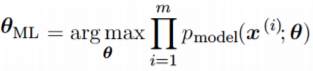
Эта произведение многих вероятностей может быть неудобным по ряду
причин. В частности, оно склонно к числовой недооценке. Кроме того, чтобы найти
максимумы/минимумы этой функции, мы должны взять производную этой функции от θ и приравнять ее к 0. Поскольку это
произведение членов, нам нужно применить правило цепочки, которое довольно
громоздко. Чтобы получить более удобную, но эквивалентную задачу оптимизации,
можно использовать логарифм вероятности, который не меняет его argmax, но
удобно превращает произведение в сумму, и поскольку логарифм – строго
возрастающая функция (функция натурального логарифма – монотонное
преобразование), это не повлияет на итоговое значение θ.
В итоге, получаем:

Два важных свойства: сходимость и
эффективность
Сходимость. По мере того, как число обучающих выборок приближается к
бесконечности, оценка максимального правдоподобия сходится к истинному значению
параметра.
Эффективность. Способ измерения того, насколько мы близки к истинному
параметру, – это ожидаемая средняя квадратичная ошибка, вычисление квадратичной
разницы между оценочными и истинными значениями параметров, где математическое
ожидание вычисляется над m обучающими выборками из данных, генерирующих
распределение. Эта параметрическая среднеквадратичная ошибка уменьшается с
увеличением m, и для
больших m нижняя
граница неравенства Крамера-Рао показывает, что ни у одной сходящейся функции оценки нет
среднеквадратичной ошибки меньше, чем у оценки максимального правдоподобия.
Именно по причине
сходимости и эффективности, оценка максимального правдоподобия часто считается
предпочтительным оценщиком для машинного обучения.
Когда количество примеров достаточно мало, чтобы привести к
переобучению, стратегии регуляризации, такие как понижающие веса, могут
использоваться для получения смещенной версии оценки максимального
правдоподобия, которая имеет меньшую дисперсию, когда данные обучения
ограничены.
Максимальная апостериорная (MAP) оценка
Согласно байесовскому подходу, можно учесть влияние предварительных
данных на выбор точечной оценки. MAP может использоваться для получения
точечной оценки ненаблюдаемой величины на основе эмпирических данных. Оценка
MAP выбирает точку максимальной апостериорной вероятности (или максимальной
плотности вероятности в более распространенном случае непрерывного θ):

где с правой стороны, log(p(x|θ)) – стандартный член
логарифмической вероятности и log(p(θ)) соответствует изначальному
распределению.
Как и при полном байесовском методе, байесовский MAP имеет преимущество
использования изначальной информации, которой нет
в обучающих данных. Эта дополнительная информация помогает уменьшить дисперсию
для точечной оценки MAP (по сравнению с оценкой MLE). Однако, это происходит ценой повышенного смещения.
Функции потерь
В большинстве обучающих сетей ошибка рассчитывается как разница
между фактическим выходным значением y и прогнозируемым выходным значением ŷ.
Функция, используемая для вычисления этой ошибки, известна как функция потерь,
также часто называемая функцией ошибки или затрат.
До сих пор наше основное внимание уделялось оценке параметров с
помощью MLE или MAP. Причина, по которой мы обсуждали это раньше, заключается в
том, что и MLE, и MAP предоставляют механизм для получения функции потерь.
Давайте рассмотрим некоторые часто используемые функции потерь.
Средняя
квадратичная ошибка (MSE): средняя
квадратичная ошибка является наиболее распространенной функцией потерь. Функция
потерь MSE широко используется в линейной регрессии в качестве показателя
эффективности. Чтобы рассчитать MSE, надо взять разницу между предсказанными
значениями и истинными, возвести ее в квадрат и усреднить по всему набору
данных.

где y(i) – фактический ожидаемый результат, а ŷ(i) – прогноз модели.
Многие функции потерь (затрат), используемые в машинном обучении,
включая MSE, могут быть получены из метода максимального правдоподобия.
Чтобы увидеть, как мы можем вывести функции потерь из MLE или MAP,
требуется некоторая математика. Вы можете пропустить ее и перейти к следующему
разделу.
Получение MSE из MLE
Алгоритм линейной регрессии учится принимать входные данные x и получать выходные значения ŷ. Отображение x в ŷ делается так,
чтобы минимизировать среднеквадратичную ошибку. Но как мы выбрали MSE в
качестве критерия для линейной регрессии? Придем к этому решению с точки зрения
оценки максимального правдоподобия. Вместо того, чтобы производить одно
предсказание ŷ , давайте рассмотрим
модель условного распределения p(y|x).
Можно смоделировать модель
линейной регрессии следующим образом:

мы предполагаем, что у имеет
нормальное распределение с ŷ в качестве
среднего значения распределения и некоторой постоянной σ² в качестве дисперсии, выбранной пользователем. Нормальное
распределения являются разумным выбором во многих случаях. В отсутствие
предварительных данных о том, какое распределение в действительности
соответствует рассматриваемым данным, нормальное распределение является хорошим
выбором по умолчанию.
Вернемся к логарифмической вероятности, определенной ранее:

где ŷ(i) – результат
линейной регрессии на i-м входе, а m – количество обучающих примеров. Мы видим,
что две первые величины являются постоянными, поэтому максимизация
логарифмической вероятности сводится к минимизации MSE:
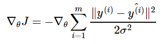
Таким образом, максимизация логарифмического правдоподобия
относительно θ дает такую же оценку параметров θ, что и минимизация
среднеквадратичной ошибки. Два критерия имеют разные значения, но одинаковое
расположение оптимума. Это оправдывает использование MSE в качестве функции
оценки максимального правдоподобия.
Кросс-энтропия
(или логарифмическая функция потерь – log loss): Кросс-энтропия измеряет расхождение между двумя вероятностными
распределениями. Если кросс-энтропия велика, это означает, что разница между
двумя распределениями велика, а если кросс-энтропия мала, то распределения
похожи друг на друга.
Кросс-энтропия определяется как:

где P – распределение истинных ответов, а Q – распределение
вероятностей прогнозов модели. Можно
показать, что функция кросс-энтропии также получается из MLE, но я не буду
утомлять вас большим количеством математики.
Давайте еще
упростим это для нашей модели с:
• N – количество наблюдений
• M – количество возможных меток класса (собака,
кошка, рыба)
• y – двоичный индикатор (0 или 1) того, является
ли метка класса C правильной классификацией для наблюдения O
• p – прогнозируемая вероятность модели
Бинарная классификация
В случае бинарной классификации (M=2),
формула имеет вид:
![]()
При двоичной классификации каждая предсказанная вероятность
сравнивается с фактическим значением класса (0 или 1), и вычисляется оценка,
которая штрафует вероятность на основе расстояния от ожидаемого значения.
Визуализация
На приведенном ниже графике показан диапазон возможных значений
логистической функции потерь с учетом истинного наблюдения (y = 1). Когда
прогнозируемая вероятность приближается к 1, логистическая функция потерь
медленно уменьшается. Однако при уменьшении прогнозируемой вероятности она быстро возрастает.
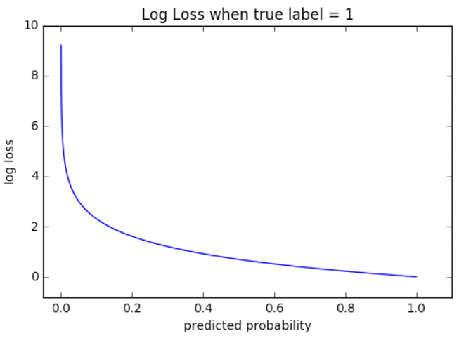
Логистическая функция потерь наказывает оба типа ошибок, но
особенно те прогнозы, которые являются достоверными и ошибочными!
Мульти-классовая классификация
В случае мульти-классовой классификации (M>2) мы берем сумму значений логарифмических функций потерь для
каждого прогноза наблюдаемых классов.
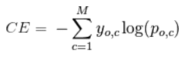
Кросс-энтропия для бинарной или двух-классовой задачи
прогнозирования фактически рассчитывается как средняя кросс-энтропия среди всех
примеров. Log loss использует отрицательные
значения логарифма, чтобы обеспечить удобную метрику для сравнения. Этот подход
основан на том, что логарифм чисел <1 возвращает отрицательные значения, что
затрудняет работу при сравнении производительности двух моделей. Вы можете
почитать эту статью, где детально обсуждается функция кросс-энтропии потерь.
Задачи ML и соответствующие функции потерь
Давайте посмотрим, какие обычно используются выходные слои и
функции потерь в задачах машинного обучения:
Задача регрессии
Задача, когда
вы прогнозируете вещественное число.
• Конфигурация выходного уровня: один
узел с линейной единицей активации.
• Функция
потерь: средняя квадратическая ошибка (MSE).
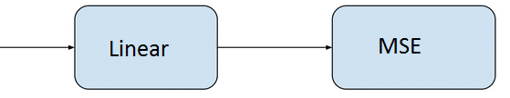
Задача бинарной классификации
Задача состоит в том, чтобы классифицировать пример как
принадлежащий одному из двух классов. Или более точно, задача сформулирована
как предсказание вероятности того, что пример принадлежит первому классу,
например, классу, которому вы присваиваете целочисленное значение 1, тогда как
другому классу присваивается значение 0.
• Конфигурация выходного
уровня: один узел с сигмовидной активационной функцией.
• Функция
потерь: кросс-энтропия, также называемая логарифмической функцией потерь.
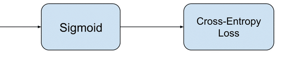
Задача мульти-классовой классификации
Эта задача состоит в том, чтобы классифицировать пример как
принадлежащий одному из нескольких классов. Задача сформулирована как
предсказание вероятности того, что пример принадлежит каждому классу.
• Конфигурация выходного уровня: один
узел для каждого класса, использующий функцию активации softmax.
• Функция потерь: кросс-энтропия, также называемая логарифмической функцией потерь.

Рассмотрев оценку и различные функции потерь, давайте перейдем к
роли оптимизаторов в алгоритмах ML.
Оптимизаторы
Чтобы свести к минимуму ошибку или потерю в прогнозировании,
модель, используя примеры из обучающей выборки, обновляет параметры модели W. Расчеты
ошибок строятся в зависимости от W и также описываются графиком функции затрат
J(w), поскольку она определяет затраты/наказание модели. Таким образом, минимизация
ошибки также часто называется минимизацией функции затрат.
Но как именно это делается? Используя оптимизаторы.
Оптимизаторы используются для обновления весов и смещений, то есть
внутренних параметров модели, чтобы уменьшить ошибку.
Самым важным методом и основой того, как мы обучаем и оптимизируем
нашу модель, является метод Градиентного Спуска.
Градиентный Спуск
Когда мы строим функцию затрат J(w), это можно представить следующим
образом:
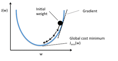
Как видно из кривой, существует значение параметров W, которое
имеет минимальное значение Jmin. Нам нужно найти способ достичь
этого минимального значения.
В алгоритме градиентного спуска мы начинаем со случайных
параметров модели и вычисляем ошибку для каждой итерации обучения, продолжая
обновлять параметры, чтобы приблизиться к минимальным значениям.
Повторяем до достижения минимума:
{

}
В приведенном выше уравнении мы обновляем параметры модели после
каждой итерации. Второй член уравнения вычисляет наклон или градиент кривой на
каждой итерации.
Градиент функции затрат вычисляется как частная производная
функции затрат J по каждому параметру модели Wj, где j принимает
значение числа признаков [1, n]. α – альфа, это скорость обучения, определяющий
как быстро мы хотим двигаться к минимуму. Если α слишком велико, мы можем
проскочить минимум. Если α слишком мало, это приведет к небольшим этапам обучения,
поэтому общее время, затрачиваемое моделью для достижения минимума, будет
больше.
Есть три способа сделать градиентный спуск:
Пакетный
градиентный спуск: использует
все обучающие данные для обновления параметров модели в каждой итерации.
Мини-пакетный градиентный спуск: вместо использования всех данных, мини-пакетный градиентный спуск делит тренировочный набор на меньший размер, называемый партией, и обозначаемый буквой «b». Таким образом, мини-пакет «b» используется для обновления параметров модели на каждой итерации.
Вот некоторые другие часто
используемые Оптимизаторы:
Стохастический
Градиентный Спуск (SGD): обновляет
параметры, используя только один обучающий параметр на каждой итерации. Такой
параметр обычно выбирается случайным образом. Стохастический градиентный спуск
часто предпочтителен для оптимизации функций затрат, когда есть сотни тысяч
обучающих или более параметров, поскольку он будет сходиться быстрее, чем
пакетный градиентный спуск.
Адаград
Адаград адаптирует скорость обучения конкретно к индивидуальным
особенностям: это означает, что некоторые веса в вашем наборе данных будут
отличаться от других. Это работает очень хорошо для разреженных наборов данных,
где пропущено много входных значений. Однако, у Адаграда есть одна серьезная
проблема: адаптивная скорость обучения со временем становится очень маленькой.
Некоторые другие оптимизаторы, описанные ниже, пытаются справиться
с этой проблемой.
RMSprop
RMSprop – это специальная версия Adagrad,
разработанная профессором Джеффри Хинтоном в его
классе нейронных сетей. Вместо того,
чтобы вычислять все градиенты, он вычисляет градиенты только в фиксированном
окне. RMSprop похож на Adaprop, это еще один оптимизатор, который пытается
решить некоторые проблемы, которые Адаград оставляет открытыми.
Адам
Адам означает адаптивную оценку момента и является еще одним способом использования
предыдущих градиентов для вычисления текущих градиентов. Адам также использует
концепцию импульса,
добавляя доли предыдущих градиентов к текущему. Этот оптимизатор получил
довольно широкое распространение и практически принят для использования в
обучающих нейронных сетях.
Вы только что ознакомились с кратким обзором
оптимизаторов. Более подробно об этом можно прочитать здесь.
Я надеюсь,
что после прочтения этой статьи, вы будете лучше понимать что происходит, когда
Вы пишите следующий код:
# loss function: Binary Cross-entropy and optimizer: Adam
model.compile(loss='binary_crossentropy', optimizer='adam')
или
# loss function: MSE and optimizer: stochastic gradient descent
model.compile(loss='mean_squared_error', optimizer='sgd')
Спасибо за проявленный интерес!
Ссылки:
[1] https://www.deeplearningbook.org/contents/ml.html
[2] https://machinelearningmastery.com/loss-and-loss-functions-for-training-deep-learning-neural-networks/
[3] https://blog.algorithmia.com/introduction-to-optimizers/
[4] https://jhui.github.io/2017/01/05/Deep-learning-Information-theory/
[5] https://blog.algorithmia.com/introduction-to-loss-functions/
[6] https://gombru.github.io/2018/05/23/cross_entropy_loss/
[7] https://www.kdnuggets.com/2018/04/right-metric-evaluating-machine-learning-models-1.html
[8] https://rohanvarma.me/Loss-Functions/
[9] http://blog.christianperone.com/2019/01/mle/