Критерий минимума среднеквадратической ошибки - Решение и исправление самых разных ошибок на TopOshibok.ru

При использовании
критерия минимума СКО, взвешивающие коэффициенты ячеек эквалайзера подстраиваются
так, чтобы минимизировать средний квадрат ошибки

, (10.2.24)

где — информационный символ,
переданный на -ом
сигнальном интервале, a — оценка этого символа на выходе
эквалайзера, определяемая (10.2.1). Если информационные символы комплексные, то
показатель качества при СКО критерия, обозначаемый , определяется так

. (10.2.25)

С другой стороны, когда
информационные символы вещественные, показатель качества просто равен квадрату
вещественной величины . В любом случае, является квадратичнйй
функцией коэффициентов эквалайзера . При дальнейшем обсуждении мы
рассмотрим минимизацию комплексной формы, даваемой (10.2.25).

Эквалайзер неограниченной
длины. Сначала
определим взвешивающие коэффициенты ячеек, которые минимизируют , когда эквалайзер
имеет неограниченное число ячеек. В этом случае, оценка определяется так

(10.2.26)

Подстановка (10.2.26) в
выражение для ,
определяемая (10.2.25), и расширение результата приводит к квадратичной функции
от коэффициентов .
Эту функцию можно легко минимизировать по посредством решения системы
(неограниченной) линейных уравнений для . Альтернативно, систему линейных
уравнений можно получить путём использования принципа ортогональности при
среднеквадратичном оценивании. Это значит, мы выбираем коэффициенты такие, что ошибка ортогональна
сигнальной

последовательности для . То есть

(10.2.27)

Подстановка в (10.2.27) даёт

или, что эквивалентно,

. (10.2.28)

Чтобы вычислить моменты в
(10.2.28), мы используем выражение для даваемое (10.1.16). Таким образом,
получим

(10.2.29)

(10.2.30)

Теперь, если подставим
(10.2.29) и (10.2.30) в (10.2.28) и возьмём -преобразование от обеих частей
результирующего уравнения, мы находим

. (10.2.31)

Следовательно,
передаточная функция эквалайзера, основанного на критерии минимума СКО, равна

. (10.2.32)

Если обеляющий фильтр
включён в ,
мы получаем эквивалентный эквалайзер с передаточной функцией

. (10.2.33)

Видим, что единственная
разница между этим выражением для и тем, которое базируется на критерии
пикового искажения — это спектральная плотность шума , которая появилась в (10.2.33),
Если очень
мало по сравнению с сигналом, коэффициенты, которые минимизируют пиковые
искажения приближённо
равны коэффициентам, которые минимизируют по СКО показатель качества . Это значит, что в
пределе, когда ,
два критерия дают одинаковое решение для взвешивающих коэффициентов. Следовательно,
когда , минимизация
СКО ведёт к полному исключению МСИ. С другой стороны, это не так, когда . В общем, когда , оба критерия дают
остаточное МСИ и аддитивный шум на выходе эквалайзера.

Меру остаточного МСИ и
аддитивного шума на выходе эквалайзера можно получить расчётом минимальной
величины ,
обозначаемую ,
когда передаточная функция

эквалайзера определена
(10.2.32). Поскольку и поскольку с учётом условия
ортогональности (10.2.27), следует

. (10.2.34)

Эта частная форма для не очень
информативна. Больше понимания зависимости качества эквалайзера от канальных
характеристик можно получить, если суммы в (10.2.34) преобразовать в частотную
область. Это можно выполнить, заметив, что сумма в (10.2.34) является свёрткой и , вычисленной при
нулевом сдвиге. Так, если через обозначить свёртку этих
последовательностей, то сумма в (10.2.34) просто равна . Поскольку — преобразование
последовательности равно

, (10.2.35)

то слагаемое равно

. (10.2.36)

Контурный интеграл в
(10.2.36) можно преобразовать в эквивалентный линейный интеграл путём замены
переменной .
В результате этой замены получаем

. (10.2.37)

Наконец, подставив (10.2.37)
в сумму (10.2.34), получаем желательное выражение для минимума СКО в виде

(10.2.38)

В отсутствие МСИ и, следовательно,

. (10.2.39)

Видим, что . Далее,
соотношение между выходным (нормированного по энергии сигнала) ОСШ и выглядит так

Более
существенно то, что соотношение и также имеет силу, когда имеется
остаточная МСИ в дополнении к шуму на выходе эквалайзера.

Эквалайзер ограниченной длины. Теперь
вернём наше внимание к случаю, когда длительность импульсной характеристики
трансверсального эквалайзера простирается на ограниченном временном интервале,
т.е. эквалайзер имеет конечную память или ограниченную длину. Выход эквалайзера
на -м сигнальном
интервале равен

СКО эквалайзера с ячейками, обозначаемый , равен

Минимизация по взвешивающим
коэффициентам ячеек или, что эквивалентно, требуя, чтобы
ошибка была
бы ортогональна сигнальным отсчётам , , приводит к следующей системе
уравнений:

где

Удобно
выразить систему линейных уравнений в матричной форме, т.е.

где означает вектор столбец взвешивающих
значений кодовых ячеек, означает матрицу ковариаций Эрмита с
элементами ;
а мерный
вектор столбец с элементами . Решение (10.2.46) можно записать в
виде

Таким образом, решение для включает в себя
обращение матрицы . Оптимальные взвешивающие
коэффициенты ячеек, даваемые (10.2.47), минимизируют показатель качества , что приводит к
минимальной величине

где определяет транспонированный вектор
столбец .
можно
использовать в (10.2.40) для вычисления ОСШ линейного эквивалента с коэффициентами
ячеек.

, (10.2.24)

. (10.2.25)

(10.2.26)

последовательности для . То есть

(10.2.27)

Подстановка в (10.2.27) даёт

или, что эквивалентно,

. (10.2.28)

Чтобы вычислить моменты в
(10.2.28), мы используем выражение для даваемое (10.1.16). Таким образом,
получим

(10.2.29)

(10.2.30)

. (10.2.31)

Следовательно,
передаточная функция эквалайзера, основанного на критерии минимума СКО, равна

. (10.2.32)

Если обеляющий фильтр
включён в ,
мы получаем эквивалентный эквалайзер с передаточной функцией

. (10.2.33)

эквалайзера определена
(10.2.32). Поскольку и поскольку с учётом условия
ортогональности (10.2.27), следует

. (10.2.34)

, (10.2.35)

то слагаемое равно

. (10.2.36)

. (10.2.37)

Наконец, подставив (10.2.37)
в сумму (10.2.34), получаем желательное выражение для минимума СКО в виде

(10.2.38)

В отсутствие МСИ и, следовательно,

. (10.2.39)

Видим, что . Далее,
соотношение между выходным (нормированного по энергии сигнала) ОСШ и выглядит так

СКО эквалайзера с ячейками, обозначаемый , равен

где

Удобно
выразить систему линейных уравнений в матричной форме, т.е.

In statistics and signal processing, a minimum mean square error (MMSE) estimator is an estimation method which minimizes the mean square error (MSE), which is a common measure of estimator quality, of the fitted values of a dependent variable. In the Bayesian setting, the term MMSE more specifically refers to estimation with quadratic loss function. In such case, the MMSE estimator is given by the posterior mean of the parameter to be estimated. Since the posterior mean is cumbersome to calculate, the form of the MMSE estimator is usually constrained to be within a certain class of functions. Linear MMSE estimators are a popular choice since they are easy to use, easy to calculate, and very versatile. It has given rise to many popular estimators such as the Wiener–Kolmogorov filter and Kalman filter.

Motivation[edit]

The term MMSE more specifically refers to estimation in a Bayesian setting with quadratic cost function. The basic idea behind the Bayesian approach to estimation stems from practical situations where we often have some prior information about the parameter to be estimated. For instance, we may have prior information about the range that the parameter can assume; or we may have an old estimate of the parameter that we want to modify when a new observation is made available; or the statistics of an actual random signal such as speech. This is in contrast to the non-Bayesian approach like minimum-variance unbiased estimator (MVUE) where absolutely nothing is assumed to be known about the parameter in advance and which does not account for such situations. In the Bayesian approach, such prior information is captured by the prior probability density function of the parameters; and based directly on Bayes theorem, it allows us to make better posterior estimates as more observations become available. Thus unlike non-Bayesian approach where parameters of interest are assumed to be deterministic, but unknown constants, the Bayesian estimator seeks to estimate a parameter that is itself a random variable. Furthermore, Bayesian estimation can also deal with situations where the sequence of observations are not necessarily independent. Thus Bayesian estimation provides yet another alternative to the MVUE. This is useful when the MVUE does not exist or cannot be found.

Definition[edit]

Let be a hidden random vector variable, and let be a known random vector variable (the measurement or observation), both of them not necessarily of the same dimension. An estimator of is any function of the measurement . The estimation error vector is given by and its mean squared error (MSE) is given by the trace of error covariance matrix

${displaystyle operatorname {MSE} =operatorname {tr} left{operatorname {E} {({hat {x}}-x)({hat {x}}-x)^{T}}right}=operatorname {E} {({hat {x}}-x)^{T}({hat {x}}-x)},}$

where the expectation is taken over conditioned on . When is a scalar variable, the MSE expression simplifies to ${displaystyle operatorname {E} left{({hat {x}}-x)^{2}right}}$ . Note that MSE can equivalently be defined in other ways, since

${displaystyle operatorname {tr} left{operatorname {E} {ee^{T}}right}=operatorname {E} left{operatorname {tr} {ee^{T}}right}=operatorname {E} {e^{T}e}=sum _{i=1}^{n}operatorname {E} {e_{i}^{2}}.}$

The MMSE estimator is then defined as the estimator achieving minimal MSE:

${displaystyle {hat {x}}_{operatorname {MMSE} }(y)=operatorname {argmin} _{hat {x}}operatorname {MSE} .}$

Properties[edit]

When the means and variances are finite, the MMSE estimator is uniquely defined^[1] and is given by:

${displaystyle {hat {x}}_{operatorname {MMSE} }(y)=operatorname {E} {xmid y}.}$

In other words, the MMSE estimator is the conditional expectation of

given the known observed value of the measurements. Also, since ${displaystyle {hat {x}}_{mathrm {MMSE} }}$

is the posterior mean, the error covariance matrix $C_{e}$

is equal to the posterior covariance ${displaystyle C_{X|Y}}$

matrix,

${displaystyle C_{e}=C_{X|Y}}$

The MMSE estimator is unbiased (under the regularity assumptions mentioned above):

${displaystyle operatorname {E} {{hat {x}}_{operatorname {MMSE} }(y)}=operatorname {E} {operatorname {E} {xmid y}}=operatorname {E} {x}.}$

The MMSE estimator is asymptotically unbiased and it converges in distribution to the normal distribution:

${displaystyle {sqrt {n}}({hat {x}}_{operatorname {MMSE} }-x)xrightarrow {d} {mathcal {N}}left(0,I^{-1}(x)right),}$

where

is the Fisher information of

. Thus, the MMSE estimator is asymptotically efficient.

${displaystyle operatorname {E} {({hat {x}}_{operatorname {MMSE} }-x)g(y)}=0}$

for all

in closed, linear subspace ${displaystyle {mathcal {V}}={g(y)mid g:mathbb {R} ^{m}rightarrow mathbb {R} ,operatorname {E} {g(y)^{2}}<+infty }}$

of the measurements. For random vectors, since the MSE for estimation of a random vector is the sum of the MSEs of the coordinates, finding the MMSE estimator of a random vector decomposes into finding the MMSE estimators of the coordinates of X separately:

${displaystyle operatorname {E} {(g_{i}^{*}(y)-x_{i})g_{j}(y)}=0,}$

for all i and j. More succinctly put, the cross-correlation between the minimum estimation error ${displaystyle {hat {x}}_{operatorname {MMSE} }-x}$

and the estimator

should be zero,

${displaystyle operatorname {E} {({hat {x}}_{operatorname {MMSE} }-x){hat {x}}^{T}}=0.}$

Linear MMSE estimator[edit]

In many cases, it is not possible to determine the analytical expression of the MMSE estimator. Two basic numerical approaches to obtain the MMSE estimate depends on either finding the conditional expectation or finding the minima of MSE. Direct numerical evaluation of the conditional expectation is computationally expensive since it often requires multidimensional integration usually done via Monte Carlo methods. Another computational approach is to directly seek the minima of the MSE using techniques such as the stochastic gradient descent methods ; but this method still requires the evaluation of expectation. While these numerical methods have been fruitful, a closed form expression for the MMSE estimator is nevertheless possible if we are willing to make some compromises.

One possibility is to abandon the full optimality requirements and seek a technique minimizing the MSE within a particular class of estimators, such as the class of linear estimators. Thus, we postulate that the conditional expectation of given is a simple linear function of , , where the measurement is a random vector, is a matrix and is a vector. This can be seen as the first order Taylor approximation of . The linear MMSE estimator is the estimator achieving minimum MSE among all estimators of such form. That is, it solves the following the optimization problem:

${displaystyle min _{W,b}operatorname {MSE} qquad {text{s.t.}}qquad {hat {x}}=Wy+b.}$

One advantage of such linear MMSE estimator is that it is not necessary to explicitly calculate the posterior probability density function of . Such linear estimator only depends on the first two moments of and . So although it may be convenient to assume that and are jointly Gaussian, it is not necessary to make this assumption, so long as the assumed distribution has well defined first and second moments. The form of the linear estimator does not depend on the type of the assumed underlying distribution.

The expression for optimal and is given by:

$W=C_{XY}C_{Y}^{-1}.$

where , the $C_{{XY}}$ is cross-covariance matrix between and , the $C_{{Y}}$ is auto-covariance matrix of .

Thus, the expression for linear MMSE estimator, its mean, and its auto-covariance is given by

${displaystyle {hat {x}}=C_{XY}C_{Y}^{-1}(y-{bar {y}})+{bar {x}},}$

{displaystyle operatorname {E} {{hat {x}}}={bar {x}},}

$C_{hat {X}}=C_{XY}C_{Y}^{-1}C_{YX},$

where the $C_{{YX}}$ is cross-covariance matrix between and .

Lastly, the error covariance and minimum mean square error achievable by such estimator is

$C_{e}=C_{X}-C_{hat {X}}=C_{X}-C_{XY}C_{Y}^{-1}C_{YX},$

${displaystyle operatorname {LMMSE} =operatorname {tr} {C_{e}}.}$

Univariate case[edit]

For the special case when both and are scalars, the above relations simplify to

${displaystyle {hat {x}}={frac {sigma _{XY}}{sigma _{Y}^{2}}}(y-{bar {y}})+{bar {x}}=rho {frac {sigma _{X}}{sigma _{Y}}}(y-{bar {y}})+{bar {x}},}$

${displaystyle sigma _{e}^{2}=sigma _{X}^{2}-{frac {sigma _{XY}^{2}}{sigma _{Y}^{2}}}=(1-rho ^{2})sigma _{X}^{2},}$

where ${displaystyle rho ={frac {sigma _{XY}}{sigma _{X}sigma _{Y}}}}$ is the Pearson’s correlation coefficient between and .

The above two equations allows us to interpret the correlation coefficient either as normalized slope of linear regression

${displaystyle left({frac {{hat {x}}-{bar {x}}}{sigma _{X}}}right)=rho left({frac {y-{bar {y}}}{sigma _{Y}}}right)}$

or as square root of the ratio of two variances

${displaystyle rho ^{2}={frac {sigma _{X}^{2}-sigma _{e}^{2}}{sigma _{X}^{2}}}={frac {sigma _{hat {X}}^{2}}{sigma _{X}^{2}}}}$

When rho =0 , we have and ${displaystyle sigma _{e}^{2}=sigma _{X}^{2}}$ . In this case, no new information is gleaned from the measurement which can decrease the uncertainty in . On the other hand, when , we have ${displaystyle {hat {x}}={frac {sigma _{XY}}{sigma _{Y}}}(y-{bar {y}})+{bar {x}}}$ and ${displaystyle sigma _{e}^{2}=0}$ . Here is completely determined by , as given by the equation of straight line.

Computation[edit]

Standard method like Gauss elimination can be used to solve the matrix equation for . A more numerically stable method is provided by QR decomposition method. Since the matrix $C_{Y}$ is a symmetric positive definite matrix, can be solved twice as fast with the Cholesky decomposition, while for large sparse systems conjugate gradient method is more effective. Levinson recursion is a fast method when $C_{Y}$ is also a Toeplitz matrix. This can happen when is a wide sense stationary process. In such stationary cases, these estimators are also referred to as Wiener–Kolmogorov filters.

Linear MMSE estimator for linear observation process[edit]

Let us further model the underlying process of observation as a linear process: y=Ax+z , where is a known matrix and is random noise vector with the mean and cross-covariance $C_{XZ}=0$ . Here the required mean and the covariance matrices will be

{displaystyle operatorname {E} {y}=A{bar {x}},}

$C_{Y}=AC_{X}A^{T}+C_{Z},$

$C_{XY}=C_{X}A^{T}.$

Thus the expression for the linear MMSE estimator matrix further modifies to

$W=C_{X}A^{T}(AC_{X}A^{T}+C_{Z})^{-1}.$

Putting everything into the expression for , we get

${hat {x}}=C_{X}A^{T}(AC_{X}A^{T}+C_{Z})^{-1}(y-A{bar {x}})+{bar {x}}.$

Lastly, the error covariance is

$C_{e}=C_{X}-C_{hat {X}}=C_{X}-C_{X}A^{T}(AC_{X}A^{T}+C_{Z})^{-1}AC_{X}.$

The significant difference between the estimation problem treated above and those of least squares and Gauss–Markov estimate is that the number of observations m, (i.e. the dimension of ) need not be at least as large as the number of unknowns, n, (i.e. the dimension of ). The estimate for the linear observation process exists so long as the m-by-m matrix $(AC_{X}A^{T}+C_{Z})^{-1}$ exists; this is the case for any m if, for instance, $C_{Z}$ is positive definite. Physically the reason for this property is that since is now a random variable, it is possible to form a meaningful estimate (namely its mean) even with no measurements. Every new measurement simply provides additional information which may modify our original estimate. Another feature of this estimate is that for m < n, there need be no measurement error. Thus, we may have $C_{Z}=0$ , because as long as $AC_{X}A^{T}$ is positive definite, the estimate still exists. Lastly, this technique can handle cases where the noise is correlated.

Alternative form[edit]

An alternative form of expression can be obtained by using the matrix identity

$C_{X}A^{T}(AC_{X}A^{T}+C_{Z})^{-1}=(A^{T}C_{Z}^{-1}A+C_{X}^{-1})^{-1}A^{T}C_{Z}^{-1},$

which can be established by post-multiplying by $(AC_{X}A^{T}+C_{Z})$ and pre-multiplying by $(A^{T}C_{Z}^{-1}A+C_{X}^{-1}),$ to obtain

$W=(A^{T}C_{Z}^{-1}A+C_{X}^{-1})^{-1}A^{T}C_{Z}^{-1},$

and

$C_{e}=(A^{T}C_{Z}^{-1}A+C_{X}^{-1})^{-1}.$

Since can now be written in terms of $C_{e}$ as $W=C_{e}A^{T}C_{Z}^{-1}$ , we get a simplified expression for as

${hat {x}}=C_{e}A^{T}C_{Z}^{-1}(y-A{bar {x}})+{bar {x}}.$

In this form the above expression can be easily compared with weighed least square and Gauss–Markov estimate. In particular, when $C_{X}^{-1}=0$ , corresponding to infinite variance of the apriori information concerning , the result $W=(A^{T}C_{Z}^{-1}A)^{-1}A^{T}C_{Z}^{-1}$ is identical to the weighed linear least square estimate with $C_{Z}^{-1}$ as the weight matrix. Moreover, if the components of are uncorrelated and have equal variance such that $C_{Z}=sigma ^{2}I,$ where is an identity matrix, then $W=(A^{T}A)^{-1}A^{T}$ is identical to the ordinary least square estimate.

Sequential linear MMSE estimation[edit]

In many real-time applications, observational data is not available in a single batch. Instead the observations are made in a sequence. One possible approach is to use the sequential observations to update an old estimate as additional data becomes available, leading to finer estimates. One crucial difference between batch estimation and sequential estimation is that sequential estimation requires an additional Markov assumption.

In the Bayesian framework, such recursive estimation is easily facilitated using Bayes’ rule. Given observations, $y_{1},ldots ,y_{k}$ , Bayes’ rule gives us the posterior density of as

${displaystyle {begin{aligned}p(x|y_{1},ldots ,y_{k})&propto p(y_{k}|x,y_{1},ldots ,y_{k-1})p(x|y_{1},ldots ,y_{k-1})&=p(y_{k}|x)p(x|y_{1},ldots ,y_{k-1}).end{aligned}}}$

The ${displaystyle p(x|y_{1},ldots ,y_{k})}$ is called the posterior density, ${displaystyle p(y_{k}|x)}$ is called the likelihood function, and ${displaystyle p(x|y_{1},ldots ,y_{k-1})}$ is the prior density of k-th time step. Note that the prior density for k-th time step is the posterior density of (k-1)-th time step. This structure allows us to formulate a recursive approach to estimation. Here we have assumed the conditional independence of $y_{k}$ from previous observations ${displaystyle y_{1},ldots ,y_{k-1}}$ given as

${displaystyle p(y_{k}|x,y_{1},ldots ,y_{k-1})=p(y_{k}|x).}$

This is the Markov assumption.

The MMSE estimate $hat{x}_k$ given the th observation is then the mean of the posterior density ${displaystyle p(x|y_{1},ldots ,y_{k})}$ . Here, we have implicitly assumed that the statistical properties of does not change with time. In other words, is stationary.

In the context of linear MMSE estimator, the formula for the estimate will have the same form as before. However, the mean and covariance matrices of and will need to be replaced by those of the prior density ${displaystyle p(x|y_{1},ldots ,y_{k-1})}$ and likelihood ${displaystyle p(y_{k}|x)}$ , respectively.

The mean and covariance matrix of the prior density ${displaystyle p(x|y_{1},ldots ,y_{k-1})}$ is given by the previous MMSE estimate, ${displaystyle {bar {x}}_{k-1}={hat {x}}_{k-1}}$ , and the error covariance matrix,

${displaystyle C_{X|Y_{1},ldots ,Y_{k-1}}=mathrm {E} [(x-{hat {x}}_{k-1})(x-{hat {x}}_{k-1})^{T}]=C_{e_{k-1}},}$

respectively, as per by the property of MMSE estimators.

Similarly, for the linear observation process, the mean and covariance matrix of the likelihood ${displaystyle p(y_{k}|x)}$ is given by ${displaystyle {bar {y}}_{k}=A{hat {x}}_{k-1}}$ and

${displaystyle {begin{aligned}C_{Y_{k}|X}&=mathrm {E} [(y_{k}-{bar {y}}_{k})(y_{k}-{bar {y}}_{k})^{T}]&=mathrm {E} [(A(x-{bar {x}}_{k-1})+z)(A(x-{bar {x}}_{k-1})+z)^{T}]&=AC_{e_{k-1}}A^{T}+C_{Z}.end{aligned}}}$

The difference between the predicted value of $y_{k}$ , as given by ${displaystyle {bar {y}}_{k}=A{hat {x}}_{k-1}}$ , and the observed value of $y_{k}$ gives the prediction error ${displaystyle {tilde {y}}_{k}=y_{k}-{bar {y}}_{k}}$ , which is also referred to as innovation. It is more convenient to represent the linear MMSE in terms of the prediction error, whose mean and covariance are ${displaystyle mathrm {E} [{tilde {y}}_{k}]=0}$ and

${displaystyle C_{{tilde {Y}}_{k}}=C_{Y_{k}|X}}$

Hence, in the estimate update formula, we should replace and $C_{X}$ by ${displaystyle {hat {x}}_{k-1}}$ and ${displaystyle C_{e_{k-1}}}$ , respectively. Also, we should replace and $C_{Y}$ by ${displaystyle {bar {y}}_{k-1}}$ and ${displaystyle C_{{tilde {Y}}_{k}}}$ . Lastly, we replace $C_{{XY}}$ by

${displaystyle {begin{aligned}C_{e_{k-1}{tilde {Y}}_{k}}&=mathrm {E} [(x-{hat {x}}_{k-1})(y_{k}-{bar {y}}_{k})^{T}]&=mathrm {E} [(x-{hat {x}}_{k-1})(A(x-{hat {x}}_{k-1})+z)^{T}]&=C_{e_{k-1}}A^{T}.end{aligned}}}$

Thus, we have the new estimate as

${displaystyle {begin{aligned}{hat {x}}_{k}&={hat {x}}_{k-1}+C_{e_{k-1}{tilde {Y}}_{k}}C_{{tilde {Y}}_{k}}^{-1}(y_{k}-{bar {y}}_{k})&={hat {x}}_{k-1}+C_{e_{k-1}}A^{T}(AC_{e_{k-1}}A^{T}+C_{Z})^{-1}(y_{k}-A{hat {x}}_{k-1})end{aligned}}}$

and the new error covariance as

${displaystyle C_{e_{k}}=C_{e_{k-1}}-C_{e_{k-1}}A^{T}(AC_{e_{k-1}}A^{T}+C_{Z})^{-1}AC_{e_{k-1}}.}$

From the point of view of linear algebra, for sequential estimation, if we have an estimate ${hat {x}}_{1}$ based on measurements generating space $Y_{1}$ , then after receiving another set of measurements, we should subtract out from these measurements that part that could be anticipated from the result of the first measurements. In other words, the updating must be based on that part of the new data which is orthogonal to the old data.

The repeated use of the above two equations as more observations become available lead to recursive estimation techniques. The expressions can be more compactly written as

${displaystyle W_{k}=C_{e_{k-1}}A^{T}(AC_{e_{k-1}}A^{T}+C_{Z})^{-1},}$

${displaystyle {hat {x}}_{k}={hat {x}}_{k-1}+W_{k}(y_{k}-A{hat {x}}_{k-1}),}$

${displaystyle C_{e_{k}}=(I-W_{k}A)C_{e_{k-1}}.}$

The matrix $W_{k}$ is often referred to as the Kalman gain factor. The alternative formulation of the above algorithm will give

${displaystyle C_{e_{k}}^{-1}=C_{e_{k-1}}^{-1}+A^{T}C_{Z}^{-1}A,}$

${displaystyle W_{k}=C_{e_{k}}A^{T}C_{Z}^{-1},}$

${displaystyle {hat {x}}_{k}={hat {x}}_{k-1}+W_{k}(y_{k}-A{hat {x}}_{k-1}),}$

The repetition of these three steps as more data becomes available leads to an iterative estimation algorithm. The generalization of this idea to non-stationary cases gives rise to the Kalman filter. The three update steps outlined above indeed form the update step of the Kalman filter.

Special case: scalar observations[edit]

As an important special case, an easy to use recursive expression can be derived when at each k-th time instant the underlying linear observation process yields a scalar such that ${displaystyle y_{k}=a_{k}^{T}x_{k}+z_{k}}$ , where $a_{k}$ is n-by-1 known column vector whose values can change with time, $x_{k}$ is n-by-1 random column vector to be estimated, and $z_{k}$ is scalar noise term with variance . After (k+1)-th observation, the direct use of above recursive equations give the expression for the estimate $hat{x}_{k+1}$ as:

${displaystyle {hat {x}}_{k+1}={hat {x}}_{k}+w_{k+1}(y_{k+1}-a_{k+1}^{T}{hat {x}}_{k})}$

where $y_{{k+1}}$ is the new scalar observation and the gain factor $w_{k+1}$ is n-by-1 column vector given by

${displaystyle w_{k+1}={frac {C_{e_{k}}a_{k+1}}{sigma _{k+1}^{2}+a_{k+1}^{T}C_{e_{k}}a_{k+1}}}.}$

The ${displaystyle C_{e_{k+1}}}$ is n-by-n error covariance matrix given by

${displaystyle C_{e_{k+1}}=(I-w_{k+1}a_{k+1}^{T})C_{e_{k}}.}$

Here, no matrix inversion is required. Also, the gain factor, $w_{k+1}$ , depends on our confidence in the new data sample, as measured by the noise variance, versus that in the previous data. The initial values of and $C_{e}$ are taken to be the mean and covariance of the aprior probability density function of .

Alternative approaches: This important special case has also given rise to many other iterative methods (or adaptive filters), such as the least mean squares filter and recursive least squares filter, that directly solves the original MSE optimization problem using stochastic gradient descents. However, since the estimation error cannot be directly observed, these methods try to minimize the mean squared prediction error ${displaystyle mathrm {E} {{tilde {y}}^{T}{tilde {y}}}}$ . For instance, in the case of scalar observations, we have the gradient ${displaystyle nabla _{hat {x}}mathrm {E} {{tilde {y}}^{2}}=-2mathrm {E} {{tilde {y}}a}.}$ Thus, the update equation for the least mean square filter is given by

${displaystyle {hat {x}}_{k+1}={hat {x}}_{k}+eta _{k}mathrm {E} {{tilde {y}}_{k}a_{k}},}$

where $eta _{k}$ is the scalar step size and the expectation is approximated by the instantaneous value ${displaystyle mathrm {E} {a_{k}{tilde {y}}_{k}}approx a_{k}{tilde {y}}_{k}}$ . As we can see, these methods bypass the need for covariance matrices.

Examples[edit]

Example 1[edit]

We shall take a linear prediction problem as an example. Let a linear combination of observed scalar random variables ${displaystyle z_{1},z_{2}}$ and ${displaystyle z_{3}}$ be used to estimate another future scalar random variable ${displaystyle z_{4}}$ such that ${displaystyle {hat {z}}_{4}=sum _{i=1}^{3}w_{i}z_{i}}$ . If the random variables ${displaystyle z=[z_{1},z_{2},z_{3},z_{4}]^{T}}$ are real Gaussian random variables with zero mean and its covariance matrix given by

${displaystyle operatorname {cov} (Z)=operatorname {E} [zz^{T}]=left[{begin{array}{cccc}1&2&3&42&5&8&93&8&6&104&9&10&15end{array}}right],}$

then our task is to find the coefficients $w_{i}$ such that it will yield an optimal linear estimate ${displaystyle {hat {z}}_{4}}$ .

In terms of the terminology developed in the previous sections, for this problem we have the observation vector ${displaystyle y=[z_{1},z_{2},z_{3}]^{T}}$ , the estimator matrix $W=[w_{1},w_{2},w_{3}]$ as a row vector, and the estimated variable ${displaystyle x=z_{4}}$ as a scalar quantity. The autocorrelation matrix $C_{Y}$ is defined as

${displaystyle C_{Y}=left[{begin{array}{ccc}E[z_{1},z_{1}]&E[z_{2},z_{1}]&E[z_{3},z_{1}]E[z_{1},z_{2}]&E[z_{2},z_{2}]&E[z_{3},z_{2}]E[z_{1},z_{3}]&E[z_{2},z_{3}]&E[z_{3},z_{3}]end{array}}right]=left[{begin{array}{ccc}1&2&32&5&83&8&6end{array}}right].}$

The cross correlation matrix $C_{{YX}}$ is defined as

${displaystyle C_{YX}=left[{begin{array}{c}E[z_{4},z_{1}]E[z_{4},z_{2}]E[z_{4},z_{3}]end{array}}right]=left[{begin{array}{c}4910end{array}}right].}$

We now solve the equation $C_{Y}W^{T}=C_{YX}$ by inverting $C_{Y}$ and pre-multiplying to get

${displaystyle C_{Y}^{-1}C_{YX}=left[{begin{array}{ccc}4.85&-1.71&-0.142-1.71&0.428&0.2857-0.142&0.2857&-0.1429end{array}}right]left[{begin{array}{c}4910end{array}}right]=left[{begin{array}{c}2.57-0.142.5714end{array}}right]=W^{T}.}$

So we have ${displaystyle w_{1}=2.57,}$ ${displaystyle w_{2}=-0.142,}$ and $w_{{3}}=.5714$
as the optimal coefficients for ${displaystyle {hat {z}}_{4}}$ . Computing the minimum
mean square error then gives ${displaystyle leftVert erightVert _{min }^{2}=operatorname {E} [z_{4}z_{4}]-WC_{YX}=15-WC_{YX}=.2857}$ .^[2] Note that it is not necessary to obtain an explicit matrix inverse of $C_{Y}$ to compute the value of . The matrix equation can be solved by well known methods such as Gauss elimination method. A shorter, non-numerical example can be found in orthogonality principle.

Example 2[edit]

Consider a vector formed by taking observations of a fixed but unknown scalar parameter disturbed by white Gaussian noise. We can describe the process by a linear equation y=1x+z , where $1=[1,1,ldots ,1]^{T}$ . Depending on context it will be clear if represents a scalar or a vector. Suppose that we know $[-x_{0},x_{0}]$ to be the range within which the value of is going to fall in. We can model our uncertainty of by an aprior uniform distribution over an interval $[-x_{0},x_{0}]$ , and thus will have variance of $sigma _{X}^{2}=x_{0}^{2}/3.$ . Let the noise vector be normally distributed as $N(0,sigma _{Z}^{2}I)$ where is an identity matrix. Also and are independent and $C_{XZ}=0$ . It is easy to see that

${displaystyle {begin{aligned}&operatorname {E} {y}=0,&C_{Y}=operatorname {E} {yy^{T}}=sigma _{X}^{2}11^{T}+sigma _{Z}^{2}I,&C_{XY}=operatorname {E} {xy^{T}}=sigma _{X}^{2}1^{T}.end{aligned}}}$

Thus, the linear MMSE estimator is given by

${begin{aligned}{hat {x}}&=C_{XY}C_{Y}^{-1}y&=sigma _{X}^{2}1^{T}(sigma _{X}^{2}11^{T}+sigma _{Z}^{2}I)^{-1}y.end{aligned}}$

We can simplify the expression by using the alternative form for as

${displaystyle {begin{aligned}{hat {x}}&=left(1^{T}{frac {1}{sigma _{Z}^{2}}}I1+{frac {1}{sigma _{X}^{2}}}right)^{-1}1^{T}{frac {1}{sigma _{Z}^{2}}}Iy&={frac {1}{sigma _{Z}^{2}}}left({frac {N}{sigma _{Z}^{2}}}+{frac {1}{sigma _{X}^{2}}}right)^{-1}1^{T}y&={frac {sigma _{X}^{2}}{sigma _{X}^{2}+sigma _{Z}^{2}/N}}{bar {y}},end{aligned}}}$

where for $y=[y_{1},y_{2},ldots ,y_{N}]^{T}$ we have ${bar {y}}={frac {1^{T}y}{N}}={frac {sum _{i=1}^{N}y_{i}}{N}}.$

Similarly, the variance of the estimator is

$sigma _{hat {X}}^{2}=C_{XY}C_{Y}^{-1}C_{YX}={Big (}{frac {sigma _{X}^{2}}{sigma _{X}^{2}+sigma _{Z}^{2}/N}}{Big )}sigma _{X}^{2}.$

Thus the MMSE of this linear estimator is

${displaystyle operatorname {LMMSE} =sigma _{X}^{2}-sigma _{hat {X}}^{2}={Big (}{frac {sigma _{Z}^{2}}{sigma _{X}^{2}+sigma _{Z}^{2}/N}}{Big )}{frac {sigma _{X}^{2}}{N}}.}$

For very large , we see that the MMSE estimator of a scalar with uniform aprior distribution can be approximated by the arithmetic average of all the observed data

${displaystyle {hat {x}}={frac {1}{N}}sum _{i=1}^{N}y_{i},}$

while the variance will be unaffected by data $sigma _{hat {X}}^{2}=sigma _{X}^{2},$ and the LMMSE of the estimate will tend to zero.

However, the estimator is suboptimal since it is constrained to be linear. Had the random variable also been Gaussian, then the estimator would have been optimal. Notice, that the form of the estimator will remain unchanged, regardless of the apriori distribution of , so long as the mean and variance of these distributions are the same.

Example 3[edit]

Consider a variation of the above example: Two candidates are standing for an election. Let the fraction of votes that a candidate will receive on an election day be Thus the fraction of votes the other candidate will receive will be 1-x. We shall take as a random variable with a uniform prior distribution over [0,1] so that its mean is and variance is $sigma _{X}^{2}=1/12.$ A few weeks before the election, two independent public opinion polls were conducted by two different pollsters. The first poll revealed that the candidate is likely to get $y_{1}$ fraction of votes. Since some error is always present due to finite sampling and the particular polling methodology adopted, the first pollster declares their estimate to have an error $z_{1}$ with zero mean and variance $sigma _{Z_{1}}^{2}.$ Similarly, the second pollster declares their estimate to be $y_{2}$ with an error $z_{2}$ with zero mean and variance $sigma _{Z_{2}}^{2}.$ Note that except for the mean and variance of the error, the error distribution is unspecified. How should the two polls be combined to obtain the voting prediction for the given candidate?

As with previous example, we have

${begin{aligned}y_{1}&=x+z_{1}y_{2}&=x+z_{2}.end{aligned}}$

Here, both the ${displaystyle operatorname {E} {y_{1}}=operatorname {E} {y_{2}}={bar {x}}=1/2}$ . Thus, we can obtain the LMMSE estimate as the linear combination of $y_{1}$ and $y_{2}$ as

${hat {x}}=w_{1}(y_{1}-{bar {x}})+w_{2}(y_{2}-{bar {x}})+{bar {x}},$

where the weights are given by

${begin{aligned}w_{1}&={frac {1/sigma _{Z_{1}}^{2}}{1/sigma _{Z_{1}}^{2}+1/sigma _{Z_{2}}^{2}+1/sigma _{X}^{2}}},w_{2}&={frac {1/sigma _{Z_{2}}^{2}}{1/sigma _{Z_{1}}^{2}+1/sigma _{Z_{2}}^{2}+1/sigma _{X}^{2}}}.end{aligned}}$

Here, since the denominator term is constant, the poll with lower error is given higher weight in order to predict the election outcome. Lastly, the variance of is given by

$sigma _{hat {X}}^{2}={frac {1/sigma _{Z_{1}}^{2}+1/sigma _{Z_{2}}^{2}}{1/sigma _{Z_{1}}^{2}+1/sigma _{Z_{2}}^{2}+1/sigma _{X}^{2}}}sigma _{X}^{2},$

which makes $sigma _{hat {X}}^{2}$ smaller than $sigma _{X}^{2}.$ Thus, the LMMSE is given by

${displaystyle mathrm {LMMSE} =sigma _{X}^{2}-sigma _{hat {X}}^{2}={frac {1}{1/sigma _{Z_{1}}^{2}+1/sigma _{Z_{2}}^{2}+1/sigma _{X}^{2}}}.}$

In general, if we have pollsters, then ${displaystyle {hat {x}}=sum _{i=1}^{N}w_{i}(y_{i}-{bar {x}})+{bar {x}},}$ where the weight for i-th pollster is given by $w_{i}={frac {1/sigma _{Z_{i}}^{2}}{sum _{i=1}^{N}1/sigma _{Z_{i}}^{2}+1/sigma _{X}^{2}}}$ and the LMMSE is given by ${displaystyle mathrm {LMMSE} ={frac {1}{sum _{i=1}^{N}1/sigma _{Z_{i}}^{2}+1/sigma _{X}^{2}}}.}$

Example 4[edit]

Suppose that a musician is playing an instrument and that the sound is received by two microphones, each of them located at two different places. Let the attenuation of sound due to distance at each microphone be $a_{1}$ and $a_{2}$ , which are assumed to be known constants. Similarly, let the noise at each microphone be $z_{1}$ and $z_{2}$ , each with zero mean and variances $sigma _{Z_{1}}^{2}$ and $sigma _{Z_{2}}^{2}$ respectively. Let denote the sound produced by the musician, which is a random variable with zero mean and variance $sigma _{X}^{2}.$ How should the recorded music from these two microphones be combined, after being synced with each other?

We can model the sound received by each microphone as

${begin{aligned}y_{1}&=a_{1}x+z_{1}y_{2}&=a_{2}x+z_{2}.end{aligned}}$

Here both the ${displaystyle operatorname {E} {y_{1}}=operatorname {E} {y_{2}}=0}$ . Thus, we can combine the two sounds as

$y=w_{1}y_{1}+w_{2}y_{2}$

where the i-th weight is given as

$w_{i}={frac {a_{i}/sigma _{Z_{i}}^{2}}{sum _{i}a_{i}^{2}/sigma _{Z_{i}}^{2}+1/sigma _{X}^{2}}}.$

Notes[edit]

^ «Mean Squared Error (MSE)». www.probabilitycourse.com. Retrieved 9 May 2017.
^ Moon and Stirling.

Motivation[edit]

Definition[edit]

${displaystyle operatorname {MSE} =operatorname {tr} left{operatorname {E} {({hat {x}}-x)({hat {x}}-x)^{T}}right}=operatorname {E} {({hat {x}}-x)^{T}({hat {x}}-x)},}$

${displaystyle operatorname {tr} left{operatorname {E} {ee^{T}}right}=operatorname {E} left{operatorname {tr} {ee^{T}}right}=operatorname {E} {e^{T}e}=sum _{i=1}^{n}operatorname {E} {e_{i}^{2}}.}$

The MMSE estimator is then defined as the estimator achieving minimal MSE:

${displaystyle {hat {x}}_{operatorname {MMSE} }(y)=operatorname {argmin} _{hat {x}}operatorname {MSE} .}$

Properties[edit]

When the means and variances are finite, the MMSE estimator is uniquely defined^[1] and is given by:

${displaystyle {hat {x}}_{operatorname {MMSE} }(y)=operatorname {E} {xmid y}.}$

In other words, the MMSE estimator is the conditional expectation of

given the known observed value of the measurements. Also, since ${displaystyle {hat {x}}_{mathrm {MMSE} }}$

is the posterior mean, the error covariance matrix $C_{e}$

is equal to the posterior covariance ${displaystyle C_{X|Y}}$

matrix,

${displaystyle C_{e}=C_{X|Y}}$

The MMSE estimator is unbiased (under the regularity assumptions mentioned above):

${displaystyle operatorname {E} {{hat {x}}_{operatorname {MMSE} }(y)}=operatorname {E} {operatorname {E} {xmid y}}=operatorname {E} {x}.}$

The MMSE estimator is asymptotically unbiased and it converges in distribution to the normal distribution:

${displaystyle {sqrt {n}}({hat {x}}_{operatorname {MMSE} }-x)xrightarrow {d} {mathcal {N}}left(0,I^{-1}(x)right),}$

where

is the Fisher information of

. Thus, the MMSE estimator is asymptotically efficient.

${displaystyle operatorname {E} {({hat {x}}_{operatorname {MMSE} }-x)g(y)}=0}$

for all

in closed, linear subspace ${displaystyle {mathcal {V}}={g(y)mid g:mathbb {R} ^{m}rightarrow mathbb {R} ,operatorname {E} {g(y)^{2}}<+infty }}$

${displaystyle operatorname {E} {(g_{i}^{*}(y)-x_{i})g_{j}(y)}=0,}$

for all i and j. More succinctly put, the cross-correlation between the minimum estimation error ${displaystyle {hat {x}}_{operatorname {MMSE} }-x}$

and the estimator

should be zero,

${displaystyle operatorname {E} {({hat {x}}_{operatorname {MMSE} }-x){hat {x}}^{T}}=0.}$

Linear MMSE estimator[edit]

${displaystyle min _{W,b}operatorname {MSE} qquad {text{s.t.}}qquad {hat {x}}=Wy+b.}$

The expression for optimal and is given by:

$W=C_{XY}C_{Y}^{-1}.$

where , the $C_{{XY}}$ is cross-covariance matrix between and , the $C_{{Y}}$ is auto-covariance matrix of .

Thus, the expression for linear MMSE estimator, its mean, and its auto-covariance is given by

${displaystyle {hat {x}}=C_{XY}C_{Y}^{-1}(y-{bar {y}})+{bar {x}},}$

$C_{hat {X}}=C_{XY}C_{Y}^{-1}C_{YX},$

where the $C_{{YX}}$ is cross-covariance matrix between and .

Lastly, the error covariance and minimum mean square error achievable by such estimator is

$C_{e}=C_{X}-C_{hat {X}}=C_{X}-C_{XY}C_{Y}^{-1}C_{YX},$

${displaystyle operatorname {LMMSE} =operatorname {tr} {C_{e}}.}$

Univariate case[edit]

For the special case when both and are scalars, the above relations simplify to

${displaystyle {hat {x}}={frac {sigma _{XY}}{sigma _{Y}^{2}}}(y-{bar {y}})+{bar {x}}=rho {frac {sigma _{X}}{sigma _{Y}}}(y-{bar {y}})+{bar {x}},}$

${displaystyle sigma _{e}^{2}=sigma _{X}^{2}-{frac {sigma _{XY}^{2}}{sigma _{Y}^{2}}}=(1-rho ^{2})sigma _{X}^{2},}$

where ${displaystyle rho ={frac {sigma _{XY}}{sigma _{X}sigma _{Y}}}}$ is the Pearson’s correlation coefficient between and .

The above two equations allows us to interpret the correlation coefficient either as normalized slope of linear regression

${displaystyle left({frac {{hat {x}}-{bar {x}}}{sigma _{X}}}right)=rho left({frac {y-{bar {y}}}{sigma _{Y}}}right)}$

or as square root of the ratio of two variances

${displaystyle rho ^{2}={frac {sigma _{X}^{2}-sigma _{e}^{2}}{sigma _{X}^{2}}}={frac {sigma _{hat {X}}^{2}}{sigma _{X}^{2}}}}$

Computation[edit]

Linear MMSE estimator for linear observation process[edit]

$C_{Y}=AC_{X}A^{T}+C_{Z},$

$C_{XY}=C_{X}A^{T}.$

Thus the expression for the linear MMSE estimator matrix further modifies to

$W=C_{X}A^{T}(AC_{X}A^{T}+C_{Z})^{-1}.$

Putting everything into the expression for , we get

${hat {x}}=C_{X}A^{T}(AC_{X}A^{T}+C_{Z})^{-1}(y-A{bar {x}})+{bar {x}}.$

Lastly, the error covariance is

$C_{e}=C_{X}-C_{hat {X}}=C_{X}-C_{X}A^{T}(AC_{X}A^{T}+C_{Z})^{-1}AC_{X}.$

Alternative form[edit]

An alternative form of expression can be obtained by using the matrix identity

$C_{X}A^{T}(AC_{X}A^{T}+C_{Z})^{-1}=(A^{T}C_{Z}^{-1}A+C_{X}^{-1})^{-1}A^{T}C_{Z}^{-1},$

which can be established by post-multiplying by $(AC_{X}A^{T}+C_{Z})$ and pre-multiplying by $(A^{T}C_{Z}^{-1}A+C_{X}^{-1}),$ to obtain

$W=(A^{T}C_{Z}^{-1}A+C_{X}^{-1})^{-1}A^{T}C_{Z}^{-1},$

and

$C_{e}=(A^{T}C_{Z}^{-1}A+C_{X}^{-1})^{-1}.$

Since can now be written in terms of $C_{e}$ as $W=C_{e}A^{T}C_{Z}^{-1}$ , we get a simplified expression for as

${hat {x}}=C_{e}A^{T}C_{Z}^{-1}(y-A{bar {x}})+{bar {x}}.$

Sequential linear MMSE estimation[edit]

In the Bayesian framework, such recursive estimation is easily facilitated using Bayes’ rule. Given observations, $y_{1},ldots ,y_{k}$ , Bayes’ rule gives us the posterior density of as

${displaystyle {begin{aligned}p(x|y_{1},ldots ,y_{k})&propto p(y_{k}|x,y_{1},ldots ,y_{k-1})p(x|y_{1},ldots ,y_{k-1})&=p(y_{k}|x)p(x|y_{1},ldots ,y_{k-1}).end{aligned}}}$

${displaystyle p(y_{k}|x,y_{1},ldots ,y_{k-1})=p(y_{k}|x).}$

This is the Markov assumption.

${displaystyle C_{X|Y_{1},ldots ,Y_{k-1}}=mathrm {E} [(x-{hat {x}}_{k-1})(x-{hat {x}}_{k-1})^{T}]=C_{e_{k-1}},}$

respectively, as per by the property of MMSE estimators.

Similarly, for the linear observation process, the mean and covariance matrix of the likelihood ${displaystyle p(y_{k}|x)}$ is given by ${displaystyle {bar {y}}_{k}=A{hat {x}}_{k-1}}$ and

${displaystyle C_{{tilde {Y}}_{k}}=C_{Y_{k}|X}}$

Thus, we have the new estimate as

and the new error covariance as

${displaystyle C_{e_{k}}=C_{e_{k-1}}-C_{e_{k-1}}A^{T}(AC_{e_{k-1}}A^{T}+C_{Z})^{-1}AC_{e_{k-1}}.}$

The repeated use of the above two equations as more observations become available lead to recursive estimation techniques. The expressions can be more compactly written as

${displaystyle W_{k}=C_{e_{k-1}}A^{T}(AC_{e_{k-1}}A^{T}+C_{Z})^{-1},}$

${displaystyle {hat {x}}_{k}={hat {x}}_{k-1}+W_{k}(y_{k}-A{hat {x}}_{k-1}),}$

${displaystyle C_{e_{k}}=(I-W_{k}A)C_{e_{k-1}}.}$

The matrix $W_{k}$ is often referred to as the Kalman gain factor. The alternative formulation of the above algorithm will give

${displaystyle C_{e_{k}}^{-1}=C_{e_{k-1}}^{-1}+A^{T}C_{Z}^{-1}A,}$

${displaystyle W_{k}=C_{e_{k}}A^{T}C_{Z}^{-1},}$

${displaystyle {hat {x}}_{k}={hat {x}}_{k-1}+W_{k}(y_{k}-A{hat {x}}_{k-1}),}$

Special case: scalar observations[edit]

${displaystyle {hat {x}}_{k+1}={hat {x}}_{k}+w_{k+1}(y_{k+1}-a_{k+1}^{T}{hat {x}}_{k})}$

where $y_{{k+1}}$ is the new scalar observation and the gain factor $w_{k+1}$ is n-by-1 column vector given by

${displaystyle w_{k+1}={frac {C_{e_{k}}a_{k+1}}{sigma _{k+1}^{2}+a_{k+1}^{T}C_{e_{k}}a_{k+1}}}.}$

The ${displaystyle C_{e_{k+1}}}$ is n-by-n error covariance matrix given by

${displaystyle C_{e_{k+1}}=(I-w_{k+1}a_{k+1}^{T})C_{e_{k}}.}$

${displaystyle {hat {x}}_{k+1}={hat {x}}_{k}+eta _{k}mathrm {E} {{tilde {y}}_{k}a_{k}},}$

Examples[edit]

Example 1[edit]

${displaystyle operatorname {cov} (Z)=operatorname {E} [zz^{T}]=left[{begin{array}{cccc}1&2&3&42&5&8&93&8&6&104&9&10&15end{array}}right],}$

then our task is to find the coefficients $w_{i}$ such that it will yield an optimal linear estimate ${displaystyle {hat {z}}_{4}}$ .

The cross correlation matrix $C_{{YX}}$ is defined as

${displaystyle C_{YX}=left[{begin{array}{c}E[z_{4},z_{1}]E[z_{4},z_{2}]E[z_{4},z_{3}]end{array}}right]=left[{begin{array}{c}4910end{array}}right].}$

We now solve the equation $C_{Y}W^{T}=C_{YX}$ by inverting $C_{Y}$ and pre-multiplying to get

Example 2[edit]

${displaystyle {begin{aligned}&operatorname {E} {y}=0,&C_{Y}=operatorname {E} {yy^{T}}=sigma _{X}^{2}11^{T}+sigma _{Z}^{2}I,&C_{XY}=operatorname {E} {xy^{T}}=sigma _{X}^{2}1^{T}.end{aligned}}}$

Thus, the linear MMSE estimator is given by

${begin{aligned}{hat {x}}&=C_{XY}C_{Y}^{-1}y&=sigma _{X}^{2}1^{T}(sigma _{X}^{2}11^{T}+sigma _{Z}^{2}I)^{-1}y.end{aligned}}$

We can simplify the expression by using the alternative form for as

where for $y=[y_{1},y_{2},ldots ,y_{N}]^{T}$ we have ${bar {y}}={frac {1^{T}y}{N}}={frac {sum _{i=1}^{N}y_{i}}{N}}.$

Similarly, the variance of the estimator is

$sigma _{hat {X}}^{2}=C_{XY}C_{Y}^{-1}C_{YX}={Big (}{frac {sigma _{X}^{2}}{sigma _{X}^{2}+sigma _{Z}^{2}/N}}{Big )}sigma _{X}^{2}.$

Thus the MMSE of this linear estimator is

${displaystyle operatorname {LMMSE} =sigma _{X}^{2}-sigma _{hat {X}}^{2}={Big (}{frac {sigma _{Z}^{2}}{sigma _{X}^{2}+sigma _{Z}^{2}/N}}{Big )}{frac {sigma _{X}^{2}}{N}}.}$

For very large , we see that the MMSE estimator of a scalar with uniform aprior distribution can be approximated by the arithmetic average of all the observed data

${displaystyle {hat {x}}={frac {1}{N}}sum _{i=1}^{N}y_{i},}$

while the variance will be unaffected by data $sigma _{hat {X}}^{2}=sigma _{X}^{2},$ and the LMMSE of the estimate will tend to zero.

Example 3[edit]

As with previous example, we have

${begin{aligned}y_{1}&=x+z_{1}y_{2}&=x+z_{2}.end{aligned}}$

Here, both the ${displaystyle operatorname {E} {y_{1}}=operatorname {E} {y_{2}}={bar {x}}=1/2}$ . Thus, we can obtain the LMMSE estimate as the linear combination of $y_{1}$ and $y_{2}$ as

${hat {x}}=w_{1}(y_{1}-{bar {x}})+w_{2}(y_{2}-{bar {x}})+{bar {x}},$

where the weights are given by

Here, since the denominator term is constant, the poll with lower error is given higher weight in order to predict the election outcome. Lastly, the variance of is given by

$sigma _{hat {X}}^{2}={frac {1/sigma _{Z_{1}}^{2}+1/sigma _{Z_{2}}^{2}}{1/sigma _{Z_{1}}^{2}+1/sigma _{Z_{2}}^{2}+1/sigma _{X}^{2}}}sigma _{X}^{2},$

which makes $sigma _{hat {X}}^{2}$ smaller than $sigma _{X}^{2}.$ Thus, the LMMSE is given by

${displaystyle mathrm {LMMSE} =sigma _{X}^{2}-sigma _{hat {X}}^{2}={frac {1}{1/sigma _{Z_{1}}^{2}+1/sigma _{Z_{2}}^{2}+1/sigma _{X}^{2}}}.}$

Example 4[edit]

We can model the sound received by each microphone as

${begin{aligned}y_{1}&=a_{1}x+z_{1}y_{2}&=a_{2}x+z_{2}.end{aligned}}$

Here both the ${displaystyle operatorname {E} {y_{1}}=operatorname {E} {y_{2}}=0}$ . Thus, we can combine the two sounds as

$y=w_{1}y_{1}+w_{2}y_{2}$

where the i-th weight is given as

$w_{i}={frac {a_{i}/sigma _{Z_{i}}^{2}}{sum _{i}a_{i}^{2}/sigma _{Z_{i}}^{2}+1/sigma _{X}^{2}}}.$

Notes[edit]

^ «Mean Squared Error (MSE)». www.probabilitycourse.com. Retrieved 9 May 2017.
^ Moon and Stirling.

Спектральная плотность вычисляется по известной корреляционной функции при помощи формул.

Вопросы
самоконтроля:

Дайте
определение спектральной плотности.
Какой
функцией является спектральная
плотность.
Как
вычисляется спектральная плотность
по известной корреляционной функции.

Лекция 59

Цель
лекции: ознакомиться
с расчетами по минимуму среднеквадратичной
ошибки случайной величины.

Задачи лекции:

Расчет
по минимуму среднеквадратичной ошибки
случайной величины.
Критерий
минимума среднеквадратичной ошибки
при одновременном действии полезного
сигнала и помехи.

Желаемый
результат:

Студенты
должны знать:

Расчет
по минимуму среднеквадратичной ошибки
случайной величины.
Критерий
минимума среднеквадратичной ошибки
при одновременном действии полезного
сигнала и помехи.

Учебный материал Расчеты по минимуму среднеквадратичной ошибки

Если
на автоматическую систему действуют
одновременно полезный сигнал и помеха,
то возникает задача оптимального расчета
системы с тем, чтобы получить наименьшую
результирующую ошибку. С точки зрения
наилучшего воспроизведения полезного
сигнала система должна иметь возможно
большую полосу пропускания, а с точки
зрения наилучшего подавления помехи
система, наоборот, должна иметь возможно
меньшую полосу пропускания. Критерием
получения оптимального решения здесь
будет минимальное значение результирующей
ошибки системы, определяемой полезным
сигналом и помехой.

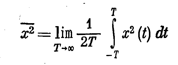
Для случайных
величин наиболее просто определить
среднеквадратичную ошибку, поэтому ее
и используют для оценки точности
автоматической системы.

Рассмотрим
расчет системы по критерию
минимума среднеквадратичной ошибки
при одновременном действии полезного
сигнала и помехи.

Согласно
этому критерию, нежелательность ошибки
пропорциональна квадрату ее величины.
Такая постановка является часто логичной,
но она не может, конечно, претендовать
на полную универсальность. В некоторых
случаях например при стрельбе по
какой-либо цели, все ошибки, большие
некоторого значения, являются одинаково
нежелательными. Однако средний квадрат
ошибки системы регулирования

практически
во всех случаях является наиболее просто
вычисляемой величиной, что и определило
использование этого критерия.

Возможны
несколько формулировок задачи. Наиболее
просто задача может быть сформулирована
так. Если имеется какая-то система
автоматического регулирования
заданной структуры, то необходимо так
выбрать параметры этой системы, чтобы
получить минимум среднеквадратичной
ошибки при заданных статистических
характеристиках полезного сигнала и
помехи.

Эта
задача решается следующим образом. По
спектральной плотности ошибки путем
ее интегрирования находится дисперсия.
Дисперсия получается зависящей от
вероятностных характеристик полезного
сигнала, помехи и параметров системы.
Затем ищутся условия, которые должны
быть наложены на параметры системы,
чтобы получить минимум дисперсии. При
достаточно простом выражении для
дисперсии это может быть определено
непосредственным дифференцированием
и приравниванием нулю частных производных.

В
более сложных случаях приходится искать
минимум дисперсии путем числового
задания интересующих параметров и
построения соответствующих графиков,
а также расчетом на ЭВМ.

Нахождение
оптимальной передаточной функции еще
не означает, что реальная автоматическая
система может быть выполнена оптимальной,
так как реализация ее может быть сопряжена
с большими трудностями. Оптимальную
передаточную функцию, за исключением
простейших случаев, следует считать
идеальной функцией, к которой по
возможности надо стремиться при
выполнении реальной автоматической
системы.

Вопросы
самоконтроля:

Какую
величину используют для оценки точности
автоматической системы со случайными
сигналами.
Дайте
определение критерию
минимума среднеквадратичной ошибки
при одновременном действии полезного
сигнала и помехи.
Как
определяется минимум
дисперсии.

Соседние файлы в папке лекции

Критерий — минимум — среднеквадратичная ошибка

Cтраница 1

Критерий минимума среднеквадратичной ошибки используется для решения более сложных задач по сравнению с задачей определения оптимальных параметров при известной структуре системы.
[1]

Идея приближения по критерию минимума среднеквадратичной ошибки, как уже указывалось, не единственна.
[2]

Тх корректирующего устройства по критерию минимума среднеквадратичной ошибки, если полезный сигнал и помеха независимы и приложены к одной точке системы.
[3]

Первое из этих условий удовлетворялось и при синтезе по критерию минимума среднеквадратичной ошибки.
[4]

Адекватность полученной модели и необходимость ее коррекции оценивают чаще всего по критерию минимума среднеквадратичной ошибки. Этот метод наиболее целесообразен.
[5]

Причем объем вычислений может быть значительно уменьшен за счет незначительного ухудшения качества, фильтрации по критерию минимума среднеквадратичной ошибки.
[6]

В большинстве практически встречающихся случаев представляется возможным, хотя бы в первом приближении, рассматривать процессы изменения технологических величин или других производственных показателей как стационарные случайные функции с нормальным распределением. Поэтому обычно критерий минимума среднеквадратичной ошибки является наиболее приемлемым в качестве критерия наилучшего предсказания в большинстве рассматриваемых задач управления.
[7]

Кроме того, по критерию минимума среднеквадратичной ошибки определяются оптимальная структура и передаточная функция замкнутой системы, обеспечивающие минимальную величину погрешности.
[8]

Анализ и синтез нелинейных систем с неизвестной структурой предлагается проводить с помощью многопеременных прямоугольных функций. Практически реализуемый алгоритм с применением этих функций получен на основе критерия минимума среднеквадратичной ошибки. Алгоритм применим при входных стационарных сигналах с произвольной плотностью распределения вероятностей.
[9]

Задача заключается в оценке значений, к-рые реализация рассматриваемого процесса ( или нек-рых его параметров, таких, как ср. Здесь в большинстве случаев определяется инвариантный во времени линейный реализуемый фильтр, оптимизирующий оценку по критерию минимума среднеквадратичной ошибки. Возможны и часто желательны др. критерии, но указанный критерий отличается математич. Для решения задач такого рода часто применяется теория Винера — Колмогорова. В этой теории предполагается, что сигнал S ( t) характеризуется только статистич. Мешающий шум N ( t) представляет также чисто случайный процесс, комбинируется с сигналом аддитивно и может быть с ним связан статистически. Далее предполагается, что накопление и обработка данных совершаются только над прошлым процессов на входе, к-рые считаются стационарными в широком смысле и имеющими положительно определенные ковариант-ные ф-ции. Кроме того, в большинстве случаев реализуются оптимальные линейные фильтры, к-рые не только реализуемы, но также и инвариантны во времени. При этих условиях импульсная переходная ф-ция линейного фильтра определяется из интегр.
[10]

Задача заключается в оценке значений, к-рые реализация рассматриваемого процесса ( или нек-рых его параметров, таких, как ср. Здесь в большинство случаев определяется инвариантный во времени линейный реализуемый фильтр, оптимизирующий оценку по критерию минимума среднеквадратичной ошибки. Возможны и часто желательны др. критерии, но указанный критерий отличается математич. Для решения задач такого рода часто применяется теория Винера — Колмогорова. В этой теории предполагается, что сигнал S ( t) характеризуется только статпстич. Мешающий шум N ( t) представляет также чисто случайный процесс, комбинируется с сигналом аддитивно и может быть с ним связан статистически. Далее предполагается, что накопление и обработка данных совершаются только над прошлым процессов па входе, к-рые считаются стационарными в широком смысле и имеющими положительно определенные ковариант-ные ф-ции. Кроме того, в большинстве случаев реализуются оптимальные линейные фильтры, к-рые не только реализуемы, но также и инвариантны во времени. При этих условиях импульсная переходная ф-ция линейного фильтра определяется из интегр.
[11]

После определения среднеквадратичной ошибки необходимо обеспечить минимальное значение ее. Наиболее просто задача решается путем минимизации среднеквадратичной ошибки по тому или иному параметру системы при заданных воздействиях. В качестве параметров, которые желательно сделать оптимальными на основе критерия минимума среднеквадратичной ошибки, могут рассматриваться различные постоянные, имеющие большое значение для определения динамических свойств системы.
[12]

Страницы:

Анализ систем на основе критерия минимума среднеквадратичной ошибки [c.189]

Если ковариационные функции процессов Х( ) и У(/) известны точно, то можно воспользоваться винеровским критерием минимума среднеквадратичной ошибки Этот критерий утверждает, что функция /г(и) должна быть выбрана так, чтобы минимизировать среднеквадратичную ошибку шумовой компоненты, т е [c.190]

Синтез следящих систем. Одно из первых инженерных применений анализа на основе критерия минимума среднеквадратичной ошибки было сделано при синтезировании следящих систем для зенитных орудий и в радиолокационных следящих системах [5] Например, от радиолокационной следящей системы требуется, чтобы она следила за самолетом несмотря на возмущения отра- [c.189]

Другое применение критерий минимума среднеквадратичной ошибки находит в задаче об идентификации системы В этом случае в распоряжении имеются входной сигнал и соответствующий ему выходной сигнал от некоторой системы, требуется вывести линейное приближение к этой системе для дальнейшего его использования при управлении или моделировании Предположим, например, что система представляет собой черный ящик (рис 5 7). Если вход является реализацией случайного процесса Х 1), то выход можно рассматривать как реализацию случайного процесса У(0< где [c.190]

Оптимальное в любом смысле корреляционное окно, например (7 2 3), будет зависеть от неизвестного спектра Гхх(/). Этот недостаток свойствен не только спектральному анализу Вообще говоря, справедливо правило, согласно которому наилучший план действий должен опираться на некоторые представления об истинном положении вещей Следовательно, очень валено проводить четкое различие между планированием спектрального анализа до сбора данных и самим анализом данных, после того как они собраны Мы хотели бы использовать критерии минимума среднеквадратичной ошибки или какой-нибудь аналогичный критерий до проведения спектрального анализа, чтобы решить, например, какой длины нужно взять запись Но после того как данные собраны, могло бы оказаться, что наши представления относительно Гхх (/) были абсолютно неправильны [c.26]

Если плотность вероятности ге ([х у) симметрична относительно среднего значения гпг [х у и унимодальна (т. е. монотонно невозрастающая функция [х — /П] [х у ), то байесовская оценка (5.18) совпадает с оценкой по критерию максимума апостериорной плотности вероятности. В этом случае функция С (х) не должна быть обязательно выпуклой, а лишь монотонно неубывающей функцией х (см. приложение С). Так как нормальная плотность вероятности унимодальна, то всегда, когда плотность вероятности ге ([х I у) нормальна, оценка по максимуму апостериорной плотности вероятности совпадает с широким классом байесовских оценок, который включает оценки по минимуму среднеквадратичной ошибки (или минимуму дисперсии). [c.158]

Анализ систем на основе критерия минимума среднеквадратичной ошибки [c.189]

From Wikipedia, the free encyclopedia

In statistics, the mean squared error (MSE)^[1] or mean squared deviation (MSD) of an estimator (of a procedure for estimating an unobserved quantity) measures the average of the squares of the errors—that is, the average squared difference between the estimated values and the actual value. MSE is a risk function, corresponding to the expected value of the squared error loss.^[2] The fact that MSE is almost always strictly positive (and not zero) is because of randomness or because the estimator does not account for information that could produce a more accurate estimate.^[3] In machine learning, specifically empirical risk minimization, MSE may refer to the empirical risk (the average loss on an observed data set), as an estimate of the true MSE (the true risk: the average loss on the actual population distribution).

The MSE is a measure of the quality of an estimator. As it is derived from the square of Euclidean distance, it is always a positive value that decreases as the error approaches zero.

The MSE is the second moment (about the origin) of the error, and thus incorporates both the variance of the estimator (how widely spread the estimates are from one data sample to another) and its bias (how far off the average estimated value is from the true value).^{[citation needed]} For an unbiased estimator, the MSE is the variance of the estimator. Like the variance, MSE has the same units of measurement as the square of the quantity being estimated. In an analogy to standard deviation, taking the square root of MSE yields the root-mean-square error or root-mean-square deviation (RMSE or RMSD), which has the same units as the quantity being estimated; for an unbiased estimator, the RMSE is the square root of the variance, known as the standard error.

Definition and basic properties[edit]

The MSE either assesses the quality of a predictor (i.e., a function mapping arbitrary inputs to a sample of values of some random variable), or of an estimator (i.e., a mathematical function mapping a sample of data to an estimate of a parameter of the population from which the data is sampled). The definition of an MSE differs according to whether one is describing a predictor or an estimator.

Predictor[edit]

If a vector of predictions is generated from a sample of data points on all variables, and is the vector of observed values of the variable being predicted, with hat{Y} being the predicted values (e.g. as from a least-squares fit), then the within-sample MSE of the predictor is computed as

${displaystyle operatorname {MSE} ={frac {1}{n}}sum _{i=1}^{n}left(Y_{i}-{hat {Y_{i}}}right)^{2}.}$

In other words, the MSE is the mean ${textstyle left({frac {1}{n}}sum _{i=1}^{n}right)}$ of the squares of the errors ${textstyle left(Y_{i}-{hat {Y_{i}}}right)^{2}}$ . This is an easily computable quantity for a particular sample (and hence is sample-dependent).

In matrix notation,

${displaystyle operatorname {MSE} ={frac {1}{n}}sum _{i=1}^{n}(e_{i})^{2}={frac {1}{n}}mathbf {e} ^{mathsf {T}}mathbf {e} }$

where $e_{i}$ is ${displaystyle (Y_{i}-{hat {Y_{i}}})}$ and is the column vector.

The MSE can also be computed on q data points that were not used in estimating the model, either because they were held back for this purpose, or because these data have been newly obtained. Within this process, known as statistical learning, the MSE is often called the test MSE,^[4] and is computed as

${displaystyle operatorname {MSE} ={frac {1}{q}}sum _{i=n+1}^{n+q}left(Y_{i}-{hat {Y_{i}}}right)^{2}.}$

Estimator[edit]

The MSE of an estimator with respect to an unknown parameter theta is defined as^[1]

${displaystyle operatorname {MSE} ({hat {theta }})=operatorname {E} _{theta }left[({hat {theta }}-theta )^{2}right].}$

This definition depends on the unknown parameter, but the MSE is a priori a property of an estimator. The MSE could be a function of unknown parameters, in which case any estimator of the MSE based on estimates of these parameters would be a function of the data (and thus a random variable). If the estimator is derived as a sample statistic and is used to estimate some population parameter, then the expectation is with respect to the sampling distribution of the sample statistic.

The MSE can be written as the sum of the variance of the estimator and the squared bias of the estimator, providing a useful way to calculate the MSE and implying that in the case of unbiased estimators, the MSE and variance are equivalent.^[5]

${displaystyle operatorname {MSE} ({hat {theta }})=operatorname {Var} _{theta }({hat {theta }})+operatorname {Bias} ({hat {theta }},theta )^{2}.}$

Proof of variance and bias relationship[edit]

${displaystyle {begin{aligned}operatorname {MSE} ({hat {theta }})&=operatorname {E} _{theta }left[({hat {theta }}-theta )^{2}right]\&=operatorname {E} _{theta }left[left({hat {theta }}-operatorname {E} _{theta }[{hat {theta }}]+operatorname {E} _{theta }[{hat {theta }}]-theta right)^{2}right]\&=operatorname {E} _{theta }left[left({hat {theta }}-operatorname {E} _{theta }[{hat {theta }}]right)^{2}+2left({hat {theta }}-operatorname {E} _{theta }[{hat {theta }}]right)left(operatorname {E} _{theta }[{hat {theta }}]-theta right)+left(operatorname {E} _{theta }[{hat {theta }}]-theta right)^{2}right]\&=operatorname {E} _{theta }left[left({hat {theta }}-operatorname {E} _{theta }[{hat {theta }}]right)^{2}right]+operatorname {E} _{theta }left[2left({hat {theta }}-operatorname {E} _{theta }[{hat {theta }}]right)left(operatorname {E} _{theta }[{hat {theta }}]-theta right)right]+operatorname {E} _{theta }left[left(operatorname {E} _{theta }[{hat {theta }}]-theta right)^{2}right]\&=operatorname {E} _{theta }left[left({hat {theta }}-operatorname {E} _{theta }[{hat {theta }}]right)^{2}right]+2left(operatorname {E} _{theta }[{hat {theta }}]-theta right)operatorname {E} _{theta }left[{hat {theta }}-operatorname {E} _{theta }[{hat {theta }}]right]+left(operatorname {E} _{theta }[{hat {theta }}]-theta right)^{2}&&operatorname {E} _{theta }[{hat {theta }}]-theta ={text{const.}}\&=operatorname {E} _{theta }left[left({hat {theta }}-operatorname {E} _{theta }[{hat {theta }}]right)^{2}right]+2left(operatorname {E} _{theta }[{hat {theta }}]-theta right)left(operatorname {E} _{theta }[{hat {theta }}]-operatorname {E} _{theta }[{hat {theta }}]right)+left(operatorname {E} _{theta }[{hat {theta }}]-theta right)^{2}&&operatorname {E} _{theta }[{hat {theta }}]={text{const.}}\&=operatorname {E} _{theta }left[left({hat {theta }}-operatorname {E} _{theta }[{hat {theta }}]right)^{2}right]+left(operatorname {E} _{theta }[{hat {theta }}]-theta right)^{2}\&=operatorname {Var} _{theta }({hat {theta }})+operatorname {Bias} _{theta }({hat {theta }},theta )^{2}end{aligned}}}$

An even shorter proof can be achieved using the well-known formula that for a random variable , ${textstyle mathbb {E} (X^{2})=operatorname {Var} (X)+(mathbb {E} (X))^{2}}$ . By substituting with, , we have

${displaystyle {begin{aligned}operatorname {MSE} ({hat {theta }})&=mathbb {E} [({hat {theta }}-theta )^{2}]\&=operatorname {Var} ({hat {theta }}-theta )+(mathbb {E} [{hat {theta }}-theta ])^{2}\&=operatorname {Var} ({hat {theta }})+operatorname {Bias} ^{2}({hat {theta }})end{aligned}}}$

But in real modeling case, MSE could be described as the addition of model variance, model bias, and irreducible uncertainty (see Bias–variance tradeoff). According to the relationship, the MSE of the estimators could be simply used for the efficiency comparison, which includes the information of estimator variance and bias. This is called MSE criterion.

In regression[edit]

In regression analysis, plotting is a more natural way to view the overall trend of the whole data. The mean of the distance from each point to the predicted regression model can be calculated, and shown as the mean squared error. The squaring is critical to reduce the complexity with negative signs. To minimize MSE, the model could be more accurate, which would mean the model is closer to actual data. One example of a linear regression using this method is the least squares method—which evaluates appropriateness of linear regression model to model bivariate dataset,^[6] but whose limitation is related to known distribution of the data.

The term mean squared error is sometimes used to refer to the unbiased estimate of error variance: the residual sum of squares divided by the number of degrees of freedom. This definition for a known, computed quantity differs from the above definition for the computed MSE of a predictor, in that a different denominator is used. The denominator is the sample size reduced by the number of model parameters estimated from the same data, (n−p) for p regressors or (n−p−1) if an intercept is used (see errors and residuals in statistics for more details).^[7] Although the MSE (as defined in this article) is not an unbiased estimator of the error variance, it is consistent, given the consistency of the predictor.

In regression analysis, «mean squared error», often referred to as mean squared prediction error or «out-of-sample mean squared error», can also refer to the mean value of the squared deviations of the predictions from the true values, over an out-of-sample test space, generated by a model estimated over a particular sample space. This also is a known, computed quantity, and it varies by sample and by out-of-sample test space.

Examples[edit]

Mean[edit]

Suppose we have a random sample of size from a population, $X_{1},dots ,X_{n}$ . Suppose the sample units were chosen with replacement. That is, the units are selected one at a time, and previously selected units are still eligible for selection for all draws. The usual estimator for the is the sample average

$overline{X}=frac{1}{n}sum_{i=1}^n X_i$

which has an expected value equal to the true mean (so it is unbiased) and a mean squared error of

${displaystyle operatorname {MSE} left({overline {X}}right)=operatorname {E} left[left({overline {X}}-mu right)^{2}right]=left({frac {sigma }{sqrt {n}}}right)^{2}={frac {sigma ^{2}}{n}}}$

where $sigma ^{2}$ is the population variance.

For a Gaussian distribution, this is the best unbiased estimator (i.e., one with the lowest MSE among all unbiased estimators), but not, say, for a uniform distribution.

Variance[edit]

The usual estimator for the variance is the corrected sample variance:

${displaystyle S_{n-1}^{2}={frac {1}{n-1}}sum _{i=1}^{n}left(X_{i}-{overline {X}}right)^{2}={frac {1}{n-1}}left(sum _{i=1}^{n}X_{i}^{2}-n{overline {X}}^{2}right).}$

This is unbiased (its expected value is $sigma ^{2}$ ), hence also called the unbiased sample variance, and its MSE is^[8]

${displaystyle operatorname {MSE} (S_{n-1}^{2})={frac {1}{n}}left(mu _{4}-{frac {n-3}{n-1}}sigma ^{4}right)={frac {1}{n}}left(gamma _{2}+{frac {2n}{n-1}}right)sigma ^{4},}$

where $mu _{4}$ is the fourth central moment of the distribution or population, and is the excess kurtosis.

However, one can use other estimators for $sigma ^{2}$ which are proportional to $S^2_{n-1}$ , and an appropriate choice can always give a lower mean squared error. If we define

${displaystyle S_{a}^{2}={frac {n-1}{a}}S_{n-1}^{2}={frac {1}{a}}sum _{i=1}^{n}left(X_{i}-{overline {X}},right)^{2}}$

then we calculate:

${displaystyle {begin{aligned}operatorname {MSE} (S_{a}^{2})&=operatorname {E} left[left({frac {n-1}{a}}S_{n-1}^{2}-sigma ^{2}right)^{2}right]\&=operatorname {E} left[{frac {(n-1)^{2}}{a^{2}}}S_{n-1}^{4}-2left({frac {n-1}{a}}S_{n-1}^{2}right)sigma ^{2}+sigma ^{4}right]\&={frac {(n-1)^{2}}{a^{2}}}operatorname {E} left[S_{n-1}^{4}right]-2left({frac {n-1}{a}}right)operatorname {E} left[S_{n-1}^{2}right]sigma ^{2}+sigma ^{4}\&={frac {(n-1)^{2}}{a^{2}}}operatorname {E} left[S_{n-1}^{4}right]-2left({frac {n-1}{a}}right)sigma ^{4}+sigma ^{4}&&operatorname {E} left[S_{n-1}^{2}right]=sigma ^{2}\&={frac {(n-1)^{2}}{a^{2}}}left({frac {gamma _{2}}{n}}+{frac {n+1}{n-1}}right)sigma ^{4}-2left({frac {n-1}{a}}right)sigma ^{4}+sigma ^{4}&&operatorname {E} left[S_{n-1}^{4}right]=operatorname {MSE} (S_{n-1}^{2})+sigma ^{4}\&={frac {n-1}{na^{2}}}left((n-1)gamma _{2}+n^{2}+nright)sigma ^{4}-2left({frac {n-1}{a}}right)sigma ^{4}+sigma ^{4}end{aligned}}}$

This is minimized when

$a=frac{(n-1)gamma_2+n^2+n}{n} = n+1+frac{n-1}{n}gamma_2.$

For a Gaussian distribution, where , this means that the MSE is minimized when dividing the sum by a=n+1 . The minimum excess kurtosis is ,^[a] which is achieved by a Bernoulli distribution with p = 1/2 (a coin flip), and the MSE is minimized for ${displaystyle a=n-1+{tfrac {2}{n}}.}$ Hence regardless of the kurtosis, we get a «better» estimate (in the sense of having a lower MSE) by scaling down the unbiased estimator a little bit; this is a simple example of a shrinkage estimator: one «shrinks» the estimator towards zero (scales down the unbiased estimator).

Further, while the corrected sample variance is the best unbiased estimator (minimum mean squared error among unbiased estimators) of variance for Gaussian distributions, if the distribution is not Gaussian, then even among unbiased estimators, the best unbiased estimator of the variance may not be $S^2_{n-1}.$

Gaussian distribution[edit]

The following table gives several estimators of the true parameters of the population, μ and σ², for the Gaussian case.^[9]

True value	Estimator	Mean squared error
	= the unbiased estimator of the population mean, $overline{X}=frac{1}{n}sum_{i=1}^n(X_i)$	$operatorname{MSE}(overline{X})=operatorname{E}((overline{X}-mu)^2)=left(frac{sigma}{sqrt{n}}right)^2$
${displaystyle theta =sigma ^{2}}$	= the unbiased estimator of the population variance, $S^2_{n-1} = frac{1}{n-1}sum_{i=1}^nleft(X_i-overline{X},right)^2$	$operatorname{MSE}(S^2_{n-1})=operatorname{E}((S^2_{n-1}-sigma^2)^2)=frac{2}{n - 1}sigma^4$
${displaystyle theta =sigma ^{2}}$	= the biased estimator of the population variance, $S^2_{n} = frac{1}{n}sum_{i=1}^nleft(X_i-overline{X},right)^2$	$operatorname{MSE}(S^2_{n})=operatorname{E}((S^2_{n}-sigma^2)^2)=frac{2n - 1}{n^2}sigma^4$
${displaystyle theta =sigma ^{2}}$	= the biased estimator of the population variance, $S^2_{n+1} = frac{1}{n+1}sum_{i=1}^nleft(X_i-overline{X},right)^2$	$operatorname{MSE}(S^2_{n+1})=operatorname{E}((S^2_{n+1}-sigma^2)^2)=frac{2}{n + 1}sigma^4$

Interpretation[edit]

An MSE of zero, meaning that the estimator predicts observations of the parameter theta with perfect accuracy, is ideal (but typically not possible).

Values of MSE may be used for comparative purposes. Two or more statistical models may be compared using their MSEs—as a measure of how well they explain a given set of observations: An unbiased estimator (estimated from a statistical model) with the smallest variance among all unbiased estimators is the best unbiased estimator or MVUE (Minimum-Variance Unbiased Estimator).

Both analysis of variance and linear regression techniques estimate the MSE as part of the analysis and use the estimated MSE to determine the statistical significance of the factors or predictors under study. The goal of experimental design is to construct experiments in such a way that when the observations are analyzed, the MSE is close to zero relative to the magnitude of at least one of the estimated treatment effects.

In one-way analysis of variance, MSE can be calculated by the division of the sum of squared errors and the degree of freedom. Also, the f-value is the ratio of the mean squared treatment and the MSE.

MSE is also used in several stepwise regression techniques as part of the determination as to how many predictors from a candidate set to include in a model for a given set of observations.

Applications[edit]

Minimizing MSE is a key criterion in selecting estimators: see minimum mean-square error. Among unbiased estimators, minimizing the MSE is equivalent to minimizing the variance, and the estimator that does this is the minimum variance unbiased estimator. However, a biased estimator may have lower MSE; see estimator bias.
In statistical modelling the MSE can represent the difference between the actual observations and the observation values predicted by the model. In this context, it is used to determine the extent to which the model fits the data as well as whether removing some explanatory variables is possible without significantly harming the model’s predictive ability.
In forecasting and prediction, the Brier score is a measure of forecast skill based on MSE.

Loss function[edit]

Squared error loss is one of the most widely used loss functions in statistics^{[citation needed]}, though its widespread use stems more from mathematical convenience than considerations of actual loss in applications. Carl Friedrich Gauss, who introduced the use of mean squared error, was aware of its arbitrariness and was in agreement with objections to it on these grounds.^[3] The mathematical benefits of mean squared error are particularly evident in its use at analyzing the performance of linear regression, as it allows one to partition the variation in a dataset into variation explained by the model and variation explained by randomness.

Criticism[edit]

The use of mean squared error without question has been criticized by the decision theorist James Berger. Mean squared error is the negative of the expected value of one specific utility function, the quadratic utility function, which may not be the appropriate utility function to use under a given set of circumstances. There are, however, some scenarios where mean squared error can serve as a good approximation to a loss function occurring naturally in an application.^[10]

Like variance, mean squared error has the disadvantage of heavily weighting outliers.^[11] This is a result of the squaring of each term, which effectively weights large errors more heavily than small ones. This property, undesirable in many applications, has led researchers to use alternatives such as the mean absolute error, or those based on the median.

Notes[edit]

^ This can be proved by Jensen’s inequality as follows. The fourth central moment is an upper bound for the square of variance, so that the least value for their ratio is one, therefore, the least value for the excess kurtosis is −2, achieved, for instance, by a Bernoulli with p=1/2.

References[edit]

^ ^a ^b «Mean Squared Error (MSE)». www.probabilitycourse.com. Retrieved 2020-09-12.
^ Bickel, Peter J.; Doksum, Kjell A. (2015). Mathematical Statistics: Basic Ideas and Selected Topics. Vol. I (Second ed.). p. 20. If we use quadratic loss, our risk function is called the mean squared error (MSE) …
^ ^a ^b Lehmann, E. L.; Casella, George (1998). Theory of Point Estimation (2nd ed.). New York: Springer. ISBN 978-0-387-98502-2. MR 1639875.
^ Gareth, James; Witten, Daniela; Hastie, Trevor; Tibshirani, Rob (2021). An Introduction to Statistical Learning: with Applications in R. Springer. ISBN 978-1071614174.
^ Wackerly, Dennis; Mendenhall, William; Scheaffer, Richard L. (2008). Mathematical Statistics with Applications (7 ed.). Belmont, CA, USA: Thomson Higher Education. ISBN 978-0-495-38508-0.
^ A modern introduction to probability and statistics : understanding why and how. Dekking, Michel, 1946-. London: Springer. 2005. ISBN 978-1-85233-896-1. OCLC 262680588.{{cite book}}: CS1 maint: others (link)
^ Steel, R.G.D, and Torrie, J. H., Principles and Procedures of Statistics with Special Reference to the Biological Sciences., McGraw Hill, 1960, page 288.
^ Mood, A.; Graybill, F.; Boes, D. (1974). Introduction to the Theory of Statistics (3rd ed.). McGraw-Hill. p. 229.
^ DeGroot, Morris H. (1980). Probability and Statistics (2nd ed.). Addison-Wesley.
^ Berger, James O. (1985). «2.4.2 Certain Standard Loss Functions». Statistical Decision Theory and Bayesian Analysis (2nd ed.). New York: Springer-Verlag. p. 60. ISBN 978-0-387-96098-2. MR 0804611.
^ Bermejo, Sergio; Cabestany, Joan (2001). «Oriented principal component analysis for large margin classifiers». Neural Networks. 14 (10): 1447–1461. doi:10.1016/S0893-6080(01)00106-X. PMID 11771723.

Спектральная плотность вычисляется по известной корреляционной функции при помощи формул.

Вопросы
самоконтроля:

Дайте
определение спектральной плотности.
Какой
функцией является спектральная
плотность.
Как
вычисляется спектральная плотность
по известной корреляционной функции.

Лекция 59

Цель
лекции: ознакомиться
с расчетами по минимуму среднеквадратичной
ошибки случайной величины.

Задачи лекции:

Расчет
по минимуму среднеквадратичной ошибки
случайной величины.
Критерий
минимума среднеквадратичной ошибки
при одновременном действии полезного
сигнала и помехи.

Желаемый
результат:

Студенты
должны знать:

Расчет
по минимуму среднеквадратичной ошибки
случайной величины.
Критерий
минимума среднеквадратичной ошибки
при одновременном действии полезного
сигнала и помехи.

Учебный материал Расчеты по минимуму среднеквадратичной ошибки

Вопросы
самоконтроля:

Какую
величину используют для оценки точности
автоматической системы со случайными
сигналами.
Дайте
определение критерию
минимума среднеквадратичной ошибки
при одновременном действии полезного
сигнала и помехи.
Как
определяется минимум
дисперсии.

Соседние файлы в папке лекции

Применим закон распределения равновероятности:

(4)

Подставляя (1) и (2) и (4) и вводя обозначения с фазой

Последовательная схема может быть
также реализована на основе СФ.

Нормальные
и аномальные ошибки.

Необходимо рассматривать

,
тогда

если ,
либо соответствует , то

Эта же задача стоит при
радиоизмерениях. И она может решаться при построении оптимального устройства, с
различными критериями.

Статистические
критерии оценки непрерывных параметров

сигнала.

Cуществуют
следующие критерии:

ü
Критерий максимума функции правдоподобия.

ü
максимальная апостериорная плотность распределения вероятности
параметра .

ü
Критерий минимума средне квадратичной ошибки.

ü
Критерий Баеса.

Распишем каждый критерий более
подробно.

Критерий максимального
правдоподобия.

оценка
максимального правдоподобия.

Критерий максимальной
апостериорной вероятности.

Рассмотрим статистическую схему:

Оценивается значение
максимального параметра.

Критерий минимальной средне
квадратичной ошибки.

Ошибки, связанные с фиксацией , не выходящие за пределы
корреляционного пика называются нормальные ошибки (инстр. ошибки,
ошибки шума).

Шумовая составляющая:

Дисперсия:

Шумовая составляющая имеет вид , но её особенность, что
количество сигнальных выбросов тем больше, чем больше шумовой уровень.

При регистрации шумовой выброс
может быть принят за сигнальный выброс. Ошибка может составить , а нормальные ошибки не выходят за
корреляционные пределы. Вероятность появления аномальных ошибок характеризует
неправильность измерения вообще.

При проектировании задают
соотношение сигнал/шум, чтобы избежать аномальных ошибок.

А среднеквадратичная ошибка
параметра .

Расчёт среднеквадратической ошибки.

Рассмотрим формулу исходя из
геометрического происхождения сигнала.

Источник

Motivation[edit]

Definition[edit]

Let be a $n\times 1$ hidden random vector variable, and let be a $m\times 1$ known random vector variable (the measurement or observation), both of them not necessarily of the same dimension. An estimator ${\hat {x}}(y)$ of is any function of the measurement . The estimation error vector is given by $e={\hat {x}}-x$ and its mean squared error (MSE) is given by the trace of error covariance matrix

$\operatorname {MSE} =\operatorname {tr} \left\{\operatorname {E} \{({\hat {x}}-x)({\hat {x}}-x)^{T}\}\right\}=\operatorname {E} \{({\hat {x}}-x)^{T}({\hat {x}}-x)\},$

where the expectation $\operatorname {E}$ is taken over conditioned on . When is a scalar variable, the MSE expression simplifies to $\operatorname {E} \left\{({\hat {x}}-x)^{2}\right\}$ . Note that MSE can equivalently be defined in other ways, since

$\operatorname {tr} \left\{\operatorname {E} \{ee^{T}\}\right\}=\operatorname {E} \left\{\operatorname {tr} \{ee^{T}\}\right\}=\operatorname {E} \{e^{T}e\}=\sum _{i=1}^{n}\operatorname {E} \{e_{i}^{2}\}.$

The MMSE estimator is then defined as the estimator achieving minimal MSE:

${\hat {x}}_{\operatorname {MMSE} }(y)=\operatorname {argmin} _{\hat {x}}\operatorname {MSE} .$

Properties[edit]

When the means and variances are finite, the MMSE estimator is uniquely defined^[1] and is given by:

${\hat {x}}_{\operatorname {MMSE} }(y)=\operatorname {E} \{x\mid y\}.$

In other words, the MMSE estimator is the conditional expectation of

given the known observed value of the measurements. Also, since ${\hat {x}}_{\mathrm {MMSE} }$

is the posterior mean, the error covariance matrix $C_{e}$

is equal to the posterior covariance $C_{X|Y}$

matrix,

$C_{e}=C_{X|Y}$

The MMSE estimator is unbiased (under the regularity assumptions mentioned above):

$\operatorname {E} \{{\hat {x}}_{\operatorname {MMSE} }(y)\}=\operatorname {E} \{\operatorname {E} \{x\mid y\}\}=\operatorname {E} \{x\}.$

The MMSE estimator is asymptotically unbiased and it converges in distribution to the normal distribution:

${\sqrt {n}}({\hat {x}}_{\operatorname {MMSE} }-x)\xrightarrow {d} {\mathcal {N}}\left(0,I^{-1}(x)\right),$

where

is the Fisher information of

. Thus, the MMSE estimator is asymptotically efficient.

$\operatorname {E} \{({\hat {x}}_{\operatorname {MMSE} }-x)g(y)\}=0$

for all

in closed, linear subspace ${\mathcal {V}}=\{g(y)\mid g:\mathbb {R} ^{m}\rightarrow \mathbb {R} ,\operatorname {E} \{g(y)^{2}\}<+\infty \}$

$\operatorname {E} \{(g_{i}^{*}(y)-x_{i})g_{j}(y)\}=0,$

for all i and j. More succinctly put, the cross-correlation between the minimum estimation error ${\hat {x}}_{\operatorname {MMSE} }-x$

and the estimator ${\hat {x}}$

should be zero,

$\operatorname {E} \{({\hat {x}}_{\operatorname {MMSE} }-x){\hat {x}}^{T}\}=0.$

Linear MMSE estimator[edit]

In many cases, it is not possible to determine the analytical expression of the MMSE estimator. Two basic numerical approaches to obtain the MMSE estimate depends on either finding the conditional expectation $\operatorname {E} \{x\mid y\}$ or finding the minima of MSE. Direct numerical evaluation of the conditional expectation is computationally expensive since it often requires multidimensional integration usually done via Monte Carlo methods. Another computational approach is to directly seek the minima of the MSE using techniques such as the stochastic gradient descent methods; but this method still requires the evaluation of expectation. While these numerical methods have been fruitful, a closed form expression for the MMSE estimator is nevertheless possible if we are willing to make some compromises.

One possibility is to abandon the full optimality requirements and seek a technique minimizing the MSE within a particular class of estimators, such as the class of linear estimators. Thus, we postulate that the conditional expectation of given is a simple linear function of , $\operatorname {E} \{x\mid y\}=Wy+b$ , where the measurement is a random vector, is a matrix and is a vector. This can be seen as the first order Taylor approximation of $\operatorname {E} \{x\mid y\}$ . The linear MMSE estimator is the estimator achieving minimum MSE among all estimators of such form. That is, it solves the following optimization problem:

$\min _{W,b}\operatorname {MSE} \qquad {\text{s.t.}}\qquad {\hat {x}}=Wy+b.$

The expression for optimal and is given by:

$b={\bar {x}}-W{\bar {y}},$

$W=C_{XY}C_{Y}^{-1}.$

where ${\bar {x}}=\operatorname {E} \{x\}$ , ${\bar {y}}=\operatorname {E} \{y\},$ the $C_{{XY}}$ is cross-covariance matrix between and , the $C_{{Y}}$ is auto-covariance matrix of .

Thus, the expression for linear MMSE estimator, its mean, and its auto-covariance is given by

${\hat {x}}=C_{XY}C_{Y}^{-1}(y-{\bar {y}})+{\bar {x}},$

$\operatorname {E} \{{\hat {x}}\}={\bar {x}},$

$C_{\hat {X}}=C_{XY}C_{Y}^{-1}C_{YX},$

where the $C_{{YX}}$ is cross-covariance matrix between and .

Lastly, the error covariance and minimum mean square error achievable by such estimator is

$C_{e}=C_{X}-C_{\hat {X}}=C_{X}-C_{XY}C_{Y}^{-1}C_{YX},$

$\operatorname {LMMSE} =\operatorname {tr} \{C_{e}\}.$

Univariate case[edit]

For the special case when both and are scalars, the above relations simplify to

${\hat {x}}={\frac {\sigma _{XY}}{\sigma _{Y}^{2}}}(y-{\bar {y}})+{\bar {x}}=\rho {\frac {\sigma _{X}}{\sigma _{Y}}}(y-{\bar {y}})+{\bar {x}},$

$\sigma _{e}^{2}=\sigma _{X}^{2}-{\frac {\sigma _{XY}^{2}}{\sigma _{Y}^{2}}}=(1-\rho ^{2})\sigma _{X}^{2},$

where $\rho ={\frac {\sigma _{XY}}{\sigma _{X}\sigma _{Y}}}$ is the Pearson’s correlation coefficient between and .

The above two equations allows us to interpret the correlation coefficient either as normalized slope of linear regression

$\left({\frac {{\hat {x}}-{\bar {x}}}{\sigma _{X}}}\right)=\rho \left({\frac {y-{\bar {y}}}{\sigma _{Y}}}\right)$

or as square root of the ratio of two variances

$\rho ^{2}={\frac {\sigma _{X}^{2}-\sigma _{e}^{2}}{\sigma _{X}^{2}}}={\frac {\sigma _{\hat {X}}^{2}}{\sigma _{X}^{2}}}$

When $\rho =0$ , we have ${\hat {x}}={\bar {x}}$ and $\sigma _{e}^{2}=\sigma _{X}^{2}$ . In this case, no new information is gleaned from the measurement which can decrease the uncertainty in . On the other hand, when $\rho =\pm 1$ , we have ${\hat {x}}={\frac {\sigma _{XY}}{\sigma _{Y}}}(y-{\bar {y}})+{\bar {x}}$ and $\sigma _{e}^{2}=0$ . Here is completely determined by , as given by the equation of straight line.

Computation[edit]

Linear MMSE estimator for linear observation process[edit]

Let us further model the underlying process of observation as a linear process: y=Ax+z , where is a known matrix and is random noise vector with the mean $\operatorname {E} \{z\}=0$ and cross-covariance $C_{XZ}=0$ . Here the required mean and the covariance matrices will be

$\operatorname {E} \{y\}=A{\bar {x}},$

$C_{Y}=AC_{X}A^{T}+C_{Z},$

$C_{XY}=C_{X}A^{T}.$

Thus the expression for the linear MMSE estimator matrix further modifies to

$W=C_{X}A^{T}(AC_{X}A^{T}+C_{Z})^{-1}.$

Putting everything into the expression for ${\hat {x}}$ , we get

${\hat {x}}=C_{X}A^{T}(AC_{X}A^{T}+C_{Z})^{-1}(y-A{\bar {x}})+{\bar {x}}.$

Lastly, the error covariance is

$C_{e}=C_{X}-C_{\hat {X}}=C_{X}-C_{X}A^{T}(AC_{X}A^{T}+C_{Z})^{-1}AC_{X}.$

Alternative form[edit]

An alternative form of expression can be obtained by using the matrix identity

$C_{X}A^{T}(AC_{X}A^{T}+C_{Z})^{-1}=(A^{T}C_{Z}^{-1}A+C_{X}^{-1})^{-1}A^{T}C_{Z}^{-1},$

which can be established by post-multiplying by $(AC_{X}A^{T}+C_{Z})$ and pre-multiplying by $(A^{T}C_{Z}^{-1}A+C_{X}^{-1}),$ to obtain

$W=(A^{T}C_{Z}^{-1}A+C_{X}^{-1})^{-1}A^{T}C_{Z}^{-1},$

and

$C_{e}=(A^{T}C_{Z}^{-1}A+C_{X}^{-1})^{-1}.$

Since can now be written in terms of $C_{e}$ as $W=C_{e}A^{T}C_{Z}^{-1}$ , we get a simplified expression for ${\hat {x}}$ as

${\hat {x}}=C_{e}A^{T}C_{Z}^{-1}(y-A{\bar {x}})+{\bar {x}}.$

In this form the above expression can be easily compared with weighed least square and Gauss–Markov estimate. In particular, when $C_{X}^{-1}=0$ , corresponding to infinite variance of the apriori information concerning , the result $W=(A^{T}C_{Z}^{-1}A)^{-1}A^{T}C_{Z}^{-1}$ is identical to the weighed linear least square estimate with $C_{Z}^{-1}$ as the weight matrix. Moreover, if the components of are uncorrelated and have equal variance such that $C_{Z}=\sigma ^{2}I,$ where is an identity matrix, then $W=(A^{T}A)^{-1}A^{T}$ is identical to the ordinary least square estimate.

Sequential linear MMSE estimation[edit]

In the Bayesian framework, such recursive estimation is easily facilitated using Bayes’ rule. Given observations, $y_{1},\ldots ,y_{k}$ , Bayes’ rule gives us the posterior density of $x_{k}$ as

${\begin{aligned}p(x_{k}|y_{1},\ldots ,y_{k})&\propto p(y_{k}|x,y_{1},\ldots ,y_{k-1})p(x_{k}|y_{1},\ldots ,y_{k-1})\\&=p(y_{k}|x_{k})p(x_{k}|y_{1},\ldots ,y_{k-1}).\end{aligned}}$

The $p(x_{k}|y_{1},\ldots ,y_{k})$ is called the posterior density, $p(y_{k}|x_{k})$ is called the likelihood function, and $p(x_{k}|y_{1},\ldots ,y_{k-1})$ is the prior density of k-th time step. Here we have assumed the conditional independence of $y_{k}$ from previous observations $y_{1},\ldots ,y_{k-1}$ given as

$p(y_{k}|x_{k},y_{1},\ldots ,y_{k-1})=p(y_{k}|x_{k}).$

This is the Markov assumption.

The MMSE estimate $\hat{x}_k$ given the k-th observation is then the mean of the posterior density $p(x_{k}|y_{1},\ldots ,y_{k})$ . With the lack of dynamical information on how the state changes with time, we will make a further stationarity assumption about the prior:

$p(x_{k}|y_{1},\ldots ,y_{k-1})=p(x_{k-1}|y_{1},\ldots ,y_{k-1}).$

Thus, the prior density for k-th time step is the posterior density of (k-1)-th time step. This structure allows us to formulate a recursive approach to estimation.

In the context of linear MMSE estimator, the formula for the estimate will have the same form as before: ${\hat {x}}=C_{XY}C_{Y}^{-1}(y-{\bar {y}})+{\bar {x}}.$ However, the mean and covariance matrices of and will need to be replaced by those of the prior density $p(x_{k}|y_{1},\ldots ,y_{k-1})$ and likelihood $p(y_{k}|x_{k})$ , respectively.

For the prior density $p(x_{k}|y_{1},\ldots ,y_{k-1})$ , its mean is given by the previous MMSE estimate,

${\bar {x}}_{k}=\mathrm {E} [x_{k}|y_{1},\ldots ,y_{k-1}]=\mathrm {E} [x_{k-1}|y_{1},\ldots ,y_{k-1}]={\hat {x}}_{k-1}$

and its covariance matrix is given by the previous error covariance matrix,

$C_{X_{k}|Y_{1},\ldots ,Y_{k-1}}=C_{X_{k-1}|Y_{1},\ldots ,Y_{k-1}}=C_{e_{k-1}},$

as per by the properties of MMSE estimators and the stationarity assumption.

Similarly, for the linear observation process, the mean of the likelihood $p(y_{k}|x_{k})$ is given by ${\bar {y}}_{k}=A{\bar {x}}_{k}=A{\hat {x}}_{k-1}$ and the covariance matrix is as before

${\begin{aligned}C_{Y_{k}|X_{k}}&=AC_{X_{k}|Y_{1},\ldots ,Y_{k-1}}A^{T}+C_{Z}=AC_{e_{k-1}}A^{T}+C_{Z}.\end{aligned}}$

The difference between the predicted value of $Y_{k}$ , as given by ${\bar {y}}_{k}=A{\hat {x}}_{k-1}$ , and its observed value $y_{k}$ gives the prediction error ${\tilde {y}}_{k}=y_{k}-{\bar {y}}_{k}$ , which is also referred to as innovation or residual. It is more convenient to represent the linear MMSE in terms of the prediction error, whose mean and covariance are $\mathrm {E} [{\tilde {y}}_{k}]=0$ and $C_{{\tilde {Y}}_{k}}=C_{Y_{k}|X_{k}}$ .

Hence, in the estimate update formula, we should replace ${\bar {x}}$ and $C_{X}$ by ${\hat {x}}_{k-1}$ and $C_{e_{k-1}}$ , respectively. Also, we should replace ${\bar {y}}$ and $C_{Y}$ by ${\bar {y}}_{k-1}$ and $C_{{\tilde {Y}}_{k}}$ . Lastly, we replace $C_{{XY}}$ by

${\begin{aligned}C_{X_{k}Y_{k}|Y_{1},\ldots ,Y_{k-1}}&=C_{e_{k-1}{\tilde {Y}}_{k}}=C_{e_{k-1}}A^{T}.\end{aligned}}$

Thus, we have the new estimate as new observation $y_{k}$ arrives as

${\begin{aligned}{\hat {x}}_{k}&={\hat {x}}_{k-1}+C_{e_{k-1}{\tilde {Y}}_{k}}C_{{\tilde {Y}}_{k}}^{-1}(y_{k}-{\bar {y}}_{k})\\&={\hat {x}}_{k-1}+C_{e_{k-1}}A^{T}(AC_{e_{k-1}}A^{T}+C_{Z})^{-1}(y_{k}-A{\hat {x}}_{k-1})\end{aligned}}$

and the new error covariance as

$C_{e_{k}}=C_{e_{k-1}}-C_{e_{k-1}}A^{T}(AC_{e_{k-1}}A^{T}+C_{Z})^{-1}AC_{e_{k-1}}.$

From the point of view of linear algebra, for sequential estimation, if we have an estimate ${\hat {x}}_{1}$ based on measurements generating space $Y_{1}$ , then after receiving another set of measurements, we should subtract out from these measurements that part that could be anticipated from the result of the first measurements. In other words, the updating must be based on that part of the new data which is orthogonal to the old data.

The repeated use of the above two equations as more observations become available lead to recursive estimation techniques. The expressions can be more compactly written as

$W_{k}=C_{e_{k-1}}A^{T}(AC_{e_{k-1}}A^{T}+C_{Z})^{-1},$

${\hat {x}}_{k}={\hat {x}}_{k-1}+W_{k}(y_{k}-A{\hat {x}}_{k-1}),$

$C_{e_{k}}=(I-W_{k}A)C_{e_{k-1}}.$

The matrix $W_{k}$ is often referred to as the Kalman gain factor. The alternative formulation of the above algorithm will give

$C_{e_{k}}^{-1}=C_{e_{k-1}}^{-1}+A^{T}C_{Z}^{-1}A,$

$W_{k}=C_{e_{k}}A^{T}C_{Z}^{-1},$

${\hat {x}}_{k}={\hat {x}}_{k-1}+W_{k}(y_{k}-A{\hat {x}}_{k-1}),$

Special case: scalar observations[edit]

As an important special case, an easy to use recursive expression can be derived when at each k-th time instant the underlying linear observation process yields a scalar such that $y_{k}=a_{k}^{T}x_{k}+z_{k}$ , where $a_{k}$ is n-by-1 known column vector whose values can change with time, $x_{k}$ is n-by-1 random column vector to be estimated, and $z_{k}$ is scalar noise term with variance $\sigma_k^2$ . After (k+1)-th observation, the direct use of above recursive equations give the expression for the estimate $\hat{x}_{k+1}$ as:

${\hat {x}}_{k+1}={\hat {x}}_{k}+w_{k+1}(y_{k+1}-a_{k+1}^{T}{\hat {x}}_{k})$

where $y_{{k+1}}$ is the new scalar observation and the gain factor $w_{k+1}$ is n-by-1 column vector given by

$w_{k+1}={\frac {C_{e_{k}}a_{k+1}}{\sigma _{k+1}^{2}+a_{k+1}^{T}C_{e_{k}}a_{k+1}}}.$

The $C_{e_{k+1}}$ is n-by-n error covariance matrix given by

$C_{e_{k+1}}=(I-w_{k+1}a_{k+1}^{T})C_{e_{k}}.$

Here, no matrix inversion is required. Also, the gain factor, $w_{k+1}$ , depends on our confidence in the new data sample, as measured by the noise variance, versus that in the previous data. The initial values of ${\hat {x}}$ and $C_{e}$ are taken to be the mean and covariance of the aprior probability density function of .

Alternative approaches: This important special case has also given rise to many other iterative methods (or adaptive filters), such as the least mean squares filter and recursive least squares filter, that directly solves the original MSE optimization problem using stochastic gradient descents. However, since the estimation error cannot be directly observed, these methods try to minimize the mean squared prediction error $\mathrm {E} \{{\tilde {y}}^{T}{\tilde {y}}\}$ . For instance, in the case of scalar observations, we have the gradient $\nabla _{\hat {x}}\mathrm {E} \{{\tilde {y}}^{2}\}=-2\mathrm {E} \{{\tilde {y}}a\}.$ Thus, the update equation for the least mean square filter is given by

${\hat {x}}_{k+1}={\hat {x}}_{k}+\eta _{k}\mathrm {E} \{{\tilde {y}}_{k}a_{k}\},$

where $\eta _{k}$ is the scalar step size and the expectation is approximated by the instantaneous value $\mathrm {E} \{a_{k}{\tilde {y}}_{k}\}\approx a_{k}{\tilde {y}}_{k}$ . As we can see, these methods bypass the need for covariance matrices.

[edit]

In many practical applications, the observation noise is uncorrelated. That is, $C_{Z}$ is a diagonal matrix. In such cases, it is advantageous to consider the components of as independent scalar measurements, rather than vector measurement. This allows us to reduce computation time by processing the $m\times 1$ measurement vector as scalar measurements. The use of scalar update formula avoids matrix inversion in the implementation of the covariance update equations, thus improving the numerical robustness against roundoff errors. The update can be implemented iteratively as:

$w_{k+1}^{(\ell )}={\frac {C_{e_{k}}^{(\ell )}A_{k+1}^{(\ell )T}}{C_{Z_{k+1}}^{(\ell )}+A_{k+1}^{(\ell )}C_{e_{k}}^{(\ell )}(A_{k+1}^{(\ell )T})}}$

$C_{e_{k+1}}^{(\ell )}=(I-w_{k+1}^{(\ell )}A_{k+1}^{(\ell )})C_{e_{k}}^{(\ell )}$

${\hat {x}}_{k+1}^{(\ell )}={\hat {x}}_{k}^{(\ell -1)}+w_{k+1}^{(\ell )}(y_{k+1}^{(\ell )}-A_{k+1}^{(\ell )}{\hat {x}}_{k}^{(\ell -1)})$

where $\ell =1,2,\ldots ,m$ , using the initial values $C_{e_{k+1}}^{(0)}=C_{e_{k}}$ and ${\hat {x}}_{k+1}^{(0)}={\hat {x}}_{k}$ . The intermediate variables $C_{Z_{k+1}}^{(\ell )}$ is the $\ell$ -th diagonal element of the $m\times m$ diagonal matrix $C_{Z_{k+1}}$ ; while $A_{k+1}^{(\ell )}$ is the $\ell$ -th row of $m\times n$ matrix $A_{{k+1}}$ . The final values are $C_{e_{k+1}}^{(m)}=C_{e_{k+1}}$ and ${\hat {x}}_{k+1}^{(m)}={\hat {x}}_{k+1}$ .

Examples[edit]

Example 1[edit]

We shall take a linear prediction problem as an example. Let a linear combination of observed scalar random variables $z_{1},z_{2}$ and $z_{3}$ be used to estimate another future scalar random variable $z_{4}$ such that ${\hat {z}}_{4}=\sum _{i=1}^{3}w_{i}z_{i}$ . If the random variables $z=[z_{1},z_{2},z_{3},z_{4}]^{T}$ are real Gaussian random variables with zero mean and its covariance matrix given by

$\operatorname {cov} (Z)=\operatorname {E} [zz^{T}]=\left[{\begin{array}{cccc}1&2&3&4\\2&5&8&9\\3&8&6&10\\4&9&10&15\end{array}}\right],$

then our task is to find the coefficients $w_{i}$ such that it will yield an optimal linear estimate ${\hat {z}}_{4}$ .

In terms of the terminology developed in the previous sections, for this problem we have the observation vector $y=[z_{1},z_{2},z_{3}]^{T}$ , the estimator matrix $W=[w_{1},w_{2},w_{3}]$ as a row vector, and the estimated variable $x=z_{4}$ as a scalar quantity. The autocorrelation matrix $C_{Y}$ is defined as

$C_{Y}=\left[{\begin{array}{ccc}E[z_{1},z_{1}]&E[z_{2},z_{1}]&E[z_{3},z_{1}]\\E[z_{1},z_{2}]&E[z_{2},z_{2}]&E[z_{3},z_{2}]\\E[z_{1},z_{3}]&E[z_{2},z_{3}]&E[z_{3},z_{3}]\end{array}}\right]=\left[{\begin{array}{ccc}1&2&3\\2&5&8\\3&8&6\end{array}}\right].$

The cross correlation matrix $C_{{YX}}$ is defined as

$C_{YX}=\left[{\begin{array}{c}E[z_{4},z_{1}]\\E[z_{4},z_{2}]\\E[z_{4},z_{3}]\end{array}}\right]=\left[{\begin{array}{c}4\\9\\10\end{array}}\right].$

We now solve the equation $C_{Y}W^{T}=C_{YX}$ by inverting $C_{Y}$ and pre-multiplying to get

$C_{Y}^{-1}C_{YX}=\left[{\begin{array}{ccc}4.85&-1.71&-0.142\\-1.71&0.428&0.2857\\-0.142&0.2857&-0.1429\end{array}}\right]\left[{\begin{array}{c}4\\9\\10\end{array}}\right]=\left[{\begin{array}{c}2.57\\-0.142\\0.5714\end{array}}\right]=W^{T}.$

So we have $w_{1}=2.57,$ $w_{2}=-0.142,$ and $w_{{3}}=.5714$
as the optimal coefficients for ${\hat {z}}_{4}$ . Computing the minimum
mean square error then gives $\left\Vert e\right\Vert _{\min }^{2}=\operatorname {E} [z_{4}z_{4}]-WC_{YX}=15-WC_{YX}=.2857$ .^[2] Note that it is not necessary to obtain an explicit matrix inverse of $C_{Y}$ to compute the value of . The matrix equation can be solved by well known methods such as Gauss elimination method. A shorter, non-numerical example can be found in orthogonality principle.

Example 2[edit]

Consider a vector formed by taking observations of a fixed but unknown scalar parameter disturbed by white Gaussian noise. We can describe the process by a linear equation y=1x+z , where $1=[1,1,\ldots ,1]^{T}$ . Depending on context it will be clear if represents a scalar or a vector. Suppose that we know $[-x_{0},x_{0}]$ to be the range within which the value of is going to fall in. We can model our uncertainty of by an aprior uniform distribution over an interval $[-x_{0},x_{0}]$ , and thus will have variance of $\sigma _{X}^{2}=x_{0}^{2}/3.$ . Let the noise vector be normally distributed as $N(0,\sigma _{Z}^{2}I)$ where is an identity matrix. Also and are independent and $C_{XZ}=0$ . It is easy to see that

${\begin{aligned}&\operatorname {E} \{y\}=0,\\&C_{Y}=\operatorname {E} \{yy^{T}\}=\sigma _{X}^{2}11^{T}+\sigma _{Z}^{2}I,\\&C_{XY}=\operatorname {E} \{xy^{T}\}=\sigma _{X}^{2}1^{T}.\end{aligned}}$

Thus, the linear MMSE estimator is given by

${\begin{aligned}{\hat {x}}&=C_{XY}C_{Y}^{-1}y\\&=\sigma _{X}^{2}1^{T}(\sigma _{X}^{2}11^{T}+\sigma _{Z}^{2}I)^{-1}y.\end{aligned}}$

We can simplify the expression by using the alternative form for as

${\begin{aligned}{\hat {x}}&=\left(1^{T}{\frac {1}{\sigma _{Z}^{2}}}I1+{\frac {1}{\sigma _{X}^{2}}}\right)^{-1}1^{T}{\frac {1}{\sigma _{Z}^{2}}}Iy\\&={\frac {1}{\sigma _{Z}^{2}}}\left({\frac {N}{\sigma _{Z}^{2}}}+{\frac {1}{\sigma _{X}^{2}}}\right)^{-1}1^{T}y\\&={\frac {\sigma _{X}^{2}}{\sigma _{X}^{2}+\sigma _{Z}^{2}/N}}{\bar {y}},\end{aligned}}$

where for $y=[y_{1},y_{2},\ldots ,y_{N}]^{T}$ we have ${\bar {y}}={\frac {1^{T}y}{N}}={\frac {\sum _{i=1}^{N}y_{i}}{N}}.$

Similarly, the variance of the estimator is

$\sigma _{\hat {X}}^{2}=C_{XY}C_{Y}^{-1}C_{YX}={\Big (}{\frac {\sigma _{X}^{2}}{\sigma _{X}^{2}+\sigma _{Z}^{2}/N}}{\Big )}\sigma _{X}^{2}.$

Thus the MMSE of this linear estimator is

$\operatorname {LMMSE} =\sigma _{X}^{2}-\sigma _{\hat {X}}^{2}={\Big (}{\frac {\sigma _{Z}^{2}}{\sigma _{X}^{2}+\sigma _{Z}^{2}/N}}{\Big )}{\frac {\sigma _{X}^{2}}{N}}.$

For very large , we see that the MMSE estimator of a scalar with uniform aprior distribution can be approximated by the arithmetic average of all the observed data

${\hat {x}}={\frac {1}{N}}\sum _{i=1}^{N}y_{i},$

while the variance will be unaffected by data $\sigma _{\hat {X}}^{2}=\sigma _{X}^{2},$ and the LMMSE of the estimate will tend to zero.

Example 3[edit]

Consider a variation of the above example: Two candidates are standing for an election. Let the fraction of votes that a candidate will receive on an election day be $x\in [0,1].$ Thus the fraction of votes the other candidate will receive will be 1-x. We shall take as a random variable with a uniform prior distribution over [0,1] so that its mean is ${\bar {x}}=1/2$ and variance is $\sigma _{X}^{2}=1/12.$ A few weeks before the election, two independent public opinion polls were conducted by two different pollsters. The first poll revealed that the candidate is likely to get $y_{1}$ fraction of votes. Since some error is always present due to finite sampling and the particular polling methodology adopted, the first pollster declares their estimate to have an error $z_{1}$ with zero mean and variance $\sigma _{Z_{1}}^{2}.$ Similarly, the second pollster declares their estimate to be $y_{2}$ with an error $z_{2}$ with zero mean and variance $\sigma _{Z_{2}}^{2}.$ Note that except for the mean and variance of the error, the error distribution is unspecified. How should the two polls be combined to obtain the voting prediction for the given candidate?

As with previous example, we have

${\begin{aligned}y_{1}&=x+z_{1}\\y_{2}&=x+z_{2}.\end{aligned}}$

Here, both the $\operatorname {E} \{y_{1}\}=\operatorname {E} \{y_{2}\}={\bar {x}}=1/2$ . Thus, we can obtain the LMMSE estimate as the linear combination of $y_{1}$ and $y_{2}$ as

${\hat {x}}=w_{1}(y_{1}-{\bar {x}})+w_{2}(y_{2}-{\bar {x}})+{\bar {x}},$

where the weights are given by

${\begin{aligned}w_{1}&={\frac {1/\sigma _{Z_{1}}^{2}}{1/\sigma _{Z_{1}}^{2}+1/\sigma _{Z_{2}}^{2}+1/\sigma _{X}^{2}}},\\w_{2}&={\frac {1/\sigma _{Z_{2}}^{2}}{1/\sigma _{Z_{1}}^{2}+1/\sigma _{Z_{2}}^{2}+1/\sigma _{X}^{2}}}.\end{aligned}}$

Here, since the denominator term is constant, the poll with lower error is given higher weight in order to predict the election outcome. Lastly, the variance of ${\hat {x}}$ is given by

$\sigma _{\hat {X}}^{2}={\frac {1/\sigma _{Z_{1}}^{2}+1/\sigma _{Z_{2}}^{2}}{1/\sigma _{Z_{1}}^{2}+1/\sigma _{Z_{2}}^{2}+1/\sigma _{X}^{2}}}\sigma _{X}^{2},$

which makes $\sigma _{\hat {X}}^{2}$ smaller than $\sigma _{X}^{2}.$ Thus, the LMMSE is given by

$\mathrm {LMMSE} =\sigma _{X}^{2}-\sigma _{\hat {X}}^{2}={\frac {1}{1/\sigma _{Z_{1}}^{2}+1/\sigma _{Z_{2}}^{2}+1/\sigma _{X}^{2}}}.$

In general, if we have pollsters, then ${\hat {x}}=\sum _{i=1}^{N}w_{i}(y_{i}-{\bar {x}})+{\bar {x}},$ where the weight for i-th pollster is given by $w_{i}={\frac {1/\sigma _{Z_{i}}^{2}}{\sum _{j=1}^{N}1/\sigma _{Z_{j}}^{2}+1/\sigma _{X}^{2}}}$ and the LMMSE is given by $\mathrm {LMMSE} ={\frac {1}{\sum _{j=1}^{N}1/\sigma _{Z_{j}}^{2}+1/\sigma _{X}^{2}}}.$

Example 4[edit]

Suppose that a musician is playing an instrument and that the sound is received by two microphones, each of them located at two different places. Let the attenuation of sound due to distance at each microphone be $a_{1}$ and $a_{2}$ , which are assumed to be known constants. Similarly, let the noise at each microphone be $z_{1}$ and $z_{2}$ , each with zero mean and variances $\sigma _{Z_{1}}^{2}$ and $\sigma _{Z_{2}}^{2}$ respectively. Let denote the sound produced by the musician, which is a random variable with zero mean and variance $\sigma _{X}^{2}.$ How should the recorded music from these two microphones be combined, after being synced with each other?

We can model the sound received by each microphone as

${\begin{aligned}y_{1}&=a_{1}x+z_{1}\\y_{2}&=a_{2}x+z_{2}.\end{aligned}}$

Here both the $\operatorname {E} \{y_{1}\}=\operatorname {E} \{y_{2}\}=0$ . Thus, we can combine the two sounds as

$y=w_{1}y_{1}+w_{2}y_{2}$

where the i-th weight is given as

$w_{i}={\frac {a_{i}/\sigma _{Z_{i}}^{2}}{\sum _{j}a_{j}^{2}/\sigma _{Z_{j}}^{2}+1/\sigma _{X}^{2}}}.$

Notes[edit]

^ «Mean Squared Error (MSE)». www.probabilitycourse.com. Retrieved 9 May 2017.
^ Moon and Stirling.

Критерий — минимум — среднеквадратичная ошибка

Cтраница 1

Идея приближения по критерию минимума среднеквадратичной ошибки, как уже указывалось, не единственна.
[2]

Первое из этих условий удовлетворялось и при синтезе по критерию минимума среднеквадратичной ошибки.
[4]

Страницы:

Анализ систем на основе критерия минимума среднеквадратичной ошибки [c.189]

достаточно простом выражении для дисперсии это может быть определено непосредственным дифференцированием и приравниванием нулю частных производных.

В более сложных случаях приходится искать минимум дисперсии путем числового задания интересующих параметров и построения соответствующих графиков.

Другая постановка задачи при расчете по критерию минимума среднеквадратичной ошибки заключается в том, что ставится вопрос о нахождении оптимальной структуры и значений параметров автоматической системы, при которых обеспечивается получение теоретического минимума среднеквадратичной ошибки при заданных вероятностных характеристиках полезного сигнала и помехи. Эта задача будет решена, если найти, например, передаточную функцию

замкнутой системы , при которой обеспечивается получение теоретического минимума среднеквадратичной ошибки.

Задача относится к категории вариационных задач. Приведем здесь некоторые результаты ее решения [120] для случая, когда полезный сигнал g (t) и помеха f (I) представляют собой центрированные стационарные случайные процессы, приложенные на входе системы. Перед системой ставится задача преобразовывать входной сигнал g (t) так, чтобы на ее выходе воспроизводилась величина h (t), связанная с g (t) некоторой формулой преобразования

тде Н (р) — преобразующий оператор.

Так, например, при получится задача интегрирования входного сигнала, при Н(р)=р — задача дифференцирования, при H(р) = 1 — задача простого воспроизведения со

сглаживанием помехи (обычная следящая система при наличии помех), при — статистическое упреждение (предсказание) и т. п.

На основании изложенного ошибку системы можно представить в виде

(11.130)

Выходная величина системы регулирования

(11.131)

где — весовая функция замкнутой системы. Подставляя (11.130) и (11.131) в формулу (11.129), получаем

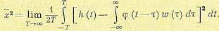(11.132)

Задача заключается в том, чтобы найти частотную передаточную функцию замкнутой системы, связанную с весовой функцией преобразованием Фурье

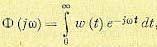(11.133)

таким образом, чтобы минимизировать значение .

Раскроем в выражении (11.132) скобки и изменим порядок интегрирования:

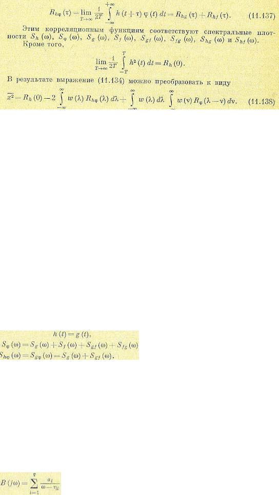
Так как в реальных системах , то нижние пределы интегрирования в (11.138) надо положить равными нулю. В результате получим

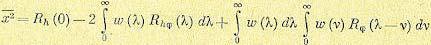(11.139)

Из последнего выражения видно, что оптимальная весовая функция, соответствующая минимуму среднего квадрата ошибки, определяется только видом корреляционных функций полезного сигнала и помехи.

Можно показать [120], что необходимое и достаточное условие минимизации выражения (11.139), которое должно быть наложено на весовую функцию, заключается в том, чтобы она была решением интегрального уравнения Винера — Хопфа

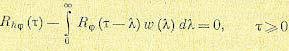(11.140)

Оптимальная передаточная функция (11.133), соответствующая оптимальной весовой функции, являющейся решением уравнения (11.140), может быть представлена в виде

(11.141)

где

(11.142)

Вчастном случае, когда преобразующий оператор Н(р) = 1, т. е в так называемом случае оптимального сглаживания, имеем

Вэтом случае решение (11.141) может быть представлено в более простом виде:

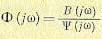(11.143)

Числитель этого выражения определяется следующим образом. Рассмотрим следующее выражение:

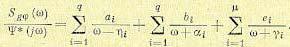(11.144)

Здесь , расположенные в верхней полуплоскости, полюсы , расположенные в нижней полуплоскости, причем полюсы предполагаются простыми, а — нули . Тогда

(11.145)

При реализации в системе оптимальной передаточной функции получится теоретический минимум среднего квадрата ошибки. Этот минимум определяется выражением или, в другом виде,

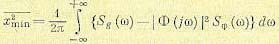(11.146)

или, в другом виде,

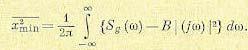(11.147).

Рассмотрим иллюстративный пример. Предположим, что полезному сигналу и помехе на входе системы регулирования соответствуют спектральные плотности:

причем корреляция между ними отсутствует и 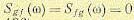. Найдем спектральную плотность, соответствующую (11.136):

Отсюда знаменатель искомой передаточной функции (11.143)

Отбросив первый член в скобках, соответствующий полюсу в нижней полуплоскости, находим числитель искомой передаточной функции (11.143):

Нахождение оптимальной передаточной функции еще не означает, что реальная автоматическая система может быть выполнена оптимальной, так как реализация ее может быть сопряжена с большими трудностями. Оптимальную передаточную функцию, за исключением простейших случаев, следует считать идеальной функцией, к которой по возможности надо стремиться при выполнении реальной автоматической системы. Теория оптимальных систем излагается в работах [26, 108, 120, 121].

ГЛАВА 12. МЕТОДЫ СИНТЕЗА СИСТЕМ АВТОМАТИЧЕСКОГО РЕГУЛИРОВАНИЯ

§ 12.1. Общие соображения

Под синтезом системы автоматического регулирования понимается направленный расчет, имеющий конечной целью отыскание рациональной структуры системы и установление оптимальных величин параметров ее отдельных звеньев. По отношению к основе синтеза в настоящее время имеются разные точки зрения.

Синтез можно трактовать как пример вариационной задачи и рассматривать такое построение системы автоматического регулирования, при котором для данных условий работы (управляющие и возмущающие воздействия, помехи, ограничения по времени работы и т. п.) обеспечивается теоретический минимум ошибки.

Синтез также можно трактовать как инженерную задачу, сводящуюся к такому построению системы автоматического регулирования, при котором обеспечивается выполнение технических требований к ней. Подразумевается, что из.многих возможных решений Инженер, проектирующий систему, будет выбирать те, которые являются оптимальными с точки зрения существующих конкретных условий и требований к габаритам, весу, простоте, надежности и т. п.

Иногда в понятие инженерного синтеза вкладывается еще более узкий смысл и рассматривается синтез, имеющий целью определение вида и параметров корректирующих средств, которые необходимо добавить к некоторой неизменяемой части системы регулирования (объект с регулятором), чтобы обеспечить требуемые динамические качества.

При инженерном синтезе системы автоматического регулирования необходимо обеспечить, во-первых, требуемую точность и, во-вторых, приемлемый характер переходных процессов.

Решение первой задачи в большинстве случаев сводится к определению требуемого общего коэффициента усиления системы и, в случае необходимости,— вида корректирующих средств, повышающих точность системы (регулирование по управляющему и возмущающему воздействиям, изодром-ные механизмы и т. п.). Эта задача может решаться при помощи определения ошибок в типовых режимах на основе тех критериев точности, которые были изложены в главе 8. Решение этой задачи, как правило, не сопряжено с трудностями принципиального или вычислительного характера, так как критерии точности достаточно просты для их практического использования. В сложных случаях можно прибегать к помощи моделирования. Решение оказывается сравнительно простым вследствие необходимости установления значений относительно небольшого числа параметров. В простейшем случае необходимо найти только общий коэффициент усиления системы.

Решение второй задачи — обеспечение приемлемых переходных процессов — оказывается почти всегда более трудным вследствие большого числа варьируемых параметров и многозначности решения задачи демпфирования системы. Поэтому существующие инженерные методы часто ограничиваются решением только второй задачи, так как их авторы считают, что обеспечение требуемой точности может быть достаточно просто сделано на основании использования существующих критериев точности и совершенствования их практически не требуется.

В настоящее время для целей синтеза систем автоматического регулирования широко используются электронные и электромеханические вычислительные машины, позволяющие производить полное или частичное моделирование проектируемой системы. При таком моделировании становится возможным наиболее полно исследовать влияние различных факторов нелинейности, зависимость параметров от времени и т. п.

Однако моделирование на вычислительных машинах не может заменить расчетных методов проектирования, которые во многих случаях позволяют исследовать вопрос в общем виде и среди многих решений найти оптимальное. Поэтому, несмотря на развитие и распространение машинных методов синтеза, теория должна располагать собственными методами, которые дополняли бы моделирование и являлись бы теоретической базой при отыскании оптимального решения.

§ 12.2. Корневой метод

Наиболее простой корневой метод разработан Т. Н. Соколовым [117]. Сущность его сводится к следующему. [В соответствии с изложенным в § 12.1 рассматривается только задача

.получения приемлемых динамических качеств при заданном значении общего коэффициента усиления, т. е. последнего члена характеристического уравнения.]

Пусть имеется характеристическое уравнение системы

(12.1)

С точки зрения скорейшего затухания переходного процесса важно, чтобы вещественные части всех корней характеристического уравнения были наибольшими. Сумма вещественных частей всех корней численно равна первому коэффициенту характеристического уравнения (12.1). Поэтому при заданной величине этого коэффициента наивыгоднейшие результаты получаются при равенстве вещественных частей всех корней/ Однако расчеты и исследования построенных систем показывают, что стремление удовлетворить поставленному требованию приводит к совершенно нереальным конструктивным характеристикам отдельных звеньев. Эти расчеты и исследования показывают, что из общего числа корней характеристического уравнения всегда можно выделить два или три корня с меньшей по абсолютному значению вещественной частью, которые и определяют ход основного процесса. Остальные же корни характеризуют быстро затухающие составляющие, оказывающие влияние только на начальной стадии переходного процесса.

Примем, что основной характер переходного процесса определяется двумя корнями. Тогда уравнение (12.1) удобно представить в виде

(12.2)

Второй сомножитель (12.2) и будет определять основной характер процесса.

Для уменьшения погрешностей проектируемой системы важно, чтобы коэффициент В2 в основном множителе имел возможно большую величину. Однако чрезмерное увеличение В2 приводит к колебательному характеру переходного процесса.

Оптимальное соотношение между коэффициентами B1 и В2 определяется из условия получения затухания за один период , которому соответствует выражение (см. §8.6)

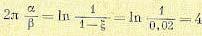(12.3)

где — вещественная и мнимая части комплексного корня, характеризующего основной процесс. Учитывая соотношения:

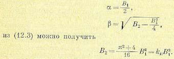(12.4)

Множитель определяющий соотношение между коэффициентами основного множителя характеристического уравнения, является критерием переходного режима, зависящим от выбранной степени затухания. Формула (12.4) показывает желаемое соотношение между коэффициентами характеристического уравнения, к которому надо стремиться при проектировании системы. Это должно осуществляться введением различных корректирующих средств.

Из (12.3) можно также получить требуемое соотношение между мнимой и вещественной частями корня (колебательность):

(12.5)

В ряде случаев для описания основного переходного процесса оказывается более целесообразным воспользоваться уравнением третьей степени

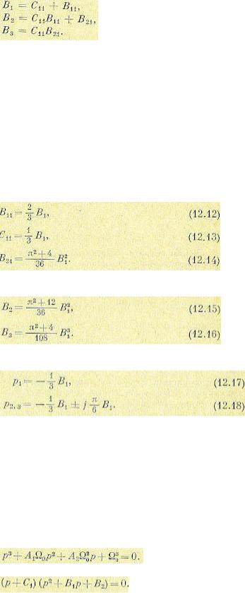
(12.6)

Это уравнение можно представить в виде

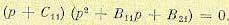(12.7)

Между коэффициентами уравнений (12.6) и (12.7) имеют место соотношения:

Положим, что во втором множителе (12.7) по-прежнему

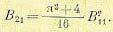(12.8)

Поэтому корни характеристического уравнения (12.6) и (12.7) равны: (12.9)

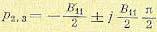(12.10)

Так как вещественная часть корней должна быть возможно большей, то целесообразно задать

(12.11)

и, следовательно,

Подставив полученные значения в формулы разложения, находим зависимость между коэффициентами основного уравнения. Если В1 задано, то

Эти соотношения должны реализоваться при проектировании системы регулирования. Корни основного уравнения

Выбор уравнения для описания основной составляющей переходного процесса зависит от структурной схемы проектируемой системы.

Рассмотрим теперь связь между основной и дополнительной составляющими переходного процесса для заданного затухания ξ (8.40). Для этой цели полезно представить характеристическое уравнение (12.1) в таком виде:

(12.19)

где — произвольно выбранный среднегеометрический корень, А1, . . . , . ., Аn-1 — безразмерные коэффициенты.

Записанное в такой форме уравнение третьей степени принимает вид

Разлагая его на множители, находим

Соотношения для коэффициентов:

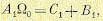(12.21)

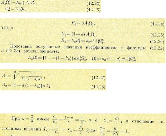
Введем коэффициент а и положим

откуда

Таким образом, безразмерные коэффициенты А1 и A2 являются функциями критерия переходного процесса &ш зависящего от. желаемой степени затухания и коэффициента разложения а, определяющего соотношение постоянных времени затухания отдельных составляющих.

Следовательно, обе составляющие переходного процесса затухают с одинаковой скоростью. Аналогичным образом можно получить выражения для коэффициентов

характеристического уравнения четвертой, пятой и более высоких степеней [117].

Синтез системы регулирования начинается с того, что для выбранной структурной схемы и введенных корректирующих средств находится характеристическое уравнение. Затем варьируются параметры основного канала регулирования и корректирующих средств таким образом, чтобы получить требуемые значения коэффициентов характеристического уравнения

(12.1) или (12.20).

Этот метод оказывается достаточно эффективным в случае сравнительно невысокой степени характеристического уравнения (n=2-4). В более сложных случаях обеспечить требуемые значения коэффициентов характеристического уравнения оказывается затруднительно, так как некоторые параметры системы и корректирующих средств могут влиять сразу на несколько коэффициентов характеристического уравнения.

Недостатком этого метода является также то, что необходимо задаваться видом корректирующих средств. Поэтому получаемое решение будет во многом зависеть от опытности проектанта.

§ 12.3. Метод корневых годографов

Качество системы регулирования с точки зрения быстродействия и запаса устойчивости может характеризоваться расположением корней числителя и знаменателя передаточной функции замкнутой системы, т. е. расположением нулей и полюсов передаточной функции (§ 8.6).

Зная эти корни, можно изобразить их расположение на комплексной плоскости корней. При расчете регулируемой системы целесообразно проследить, как меняется общая картина расположения корней при изменении отдельных параметров, например общего коэффициента усиления, постоянных времени корректирующих цепей и т. п., с целью установления оптимальных значений этих параметров.

При плавном изменении значения какого-либо параметра корни будут перемещаться на плоскости корней, прочерчивая некоторую кривую, которую будем называть корневым

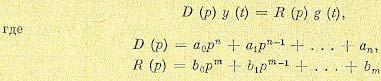
годографом или траекторией корней. Построив траектории всех корней, можно выбрать такое значение варьируемого параметра, которое соответствует наилучшему расположению корней.

Первый способ построения траекторий корней заключается в следующем. Пусть имеется дифференциальное уравнение замкнутой системы, записанное для регулируемой величины при наличии задающего воздействия (5.3):

Это уравнение записано здесь для случая равенства нулю возмущающих воздействий. Оно может быть записано также для любого возмущающего-воздействия. Это не изменит его формы и не отразится на дальнейших рассуждениях.

Передаточная функция замкнутой системы

(12.29)

Полюсы передаточной функции, т. е. корни знаменателя, обозначим через , а

ее нули (корни числителя) —через .

Коэффициенты числителя и знаменателя (12.29) определенным образом выражены через параметры регулируемого объекта, регулятора и корректирующих устройств. Если нужно

выбрать величину какого-либо параметра (постоянная времени, коэффициент усиления и т. п.), входящего как угодно в коэффициенты (12.29), то необходимо принять некоторые постоянные

значения для всех остальных параметров, а для искомого параметра задавать различные

числовые значения внутри реально возможных пределов изменения этого параметра в данной системе регулирования. Для каждого из этих вариантов необходимо затем вычислить корни числителя и знаменателя (12.29). Результаты вычислений можно свести в таблицу, на основании которой легко строятся все траектории корней.

Если нужно выбрать два или несколько параметров регулируемой системы, то такого рода вычисления нужно проделать несколько раз, меняя каждый раз один из параметров при заданных значениях всех остальных.

Вычисление корней при этом можно производить любым численным методом, возможно более простым, так как ввиду приближенности корневой оценки здесь не требуется большой точности вычислений. В настоящее время имеются электрические устройства, позволяющие строить на экране траектории корней непосредственно по заданным коэффициентам уравнения.

Из простых численных методов определения корней можно рекомендовать, например, метод последовательных делений [98].

Другой способ построения траекторий корней, разработанный Ивэнсом и Э. Г. Удерманом [128], в отличие от первого, пригодного для выбора любого параметра системы, специально приспособлен для выбора общего коэффициента усиления передаточной функции разомкнутой системы (5.10), которую запишем следующим образом:

(12.30)

Здесь К = Кr — общий коэффициент усиления разомкнутой системы, имеющий размерность сек-r, где r — степень астатизма; G1 (р) — операторная часть передаточной функции разомкнутой системы.

Характеристическое уравнение системы может быть записано в виде

(12.31)

Обозначим полюсы и нули передаточной функции разомкнутой системы соответственно через . Тогда

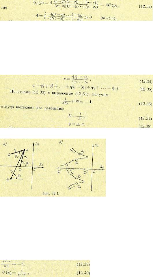
Каждый сомножитель в выражении (12.32) можно изобразить в виде вектора на комплексной плоскости (рис. 12.1), где р — текущая точка. Обозначим длину (модуль) каждого

вектора в знаменателе (12.32) через 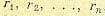, а в числителе — через Соответственно угол между вектором и положительным направлением оси вещественных

(аргумент) для знаменателя обозначим , а для числителя — . По правилу перемножения комплексных чисел согласно формуле (12.32) найдем, что G (р) будет представлять собой вектор с длиной г ж аргументом ф, причем

(12.33)

где

Траектории корней (рис. 12.1) строятся таким образом, чтобы они удовлетворяли условию (12.38). После этого по формуле (12.34) для каждой

конкретной комбинации корней можно вычислить А и величину r, а затем по формуле (12.37) — общий коэффициент усиления К.

Для упрощения построения траекторий корней используются следующие свойства. 1.При К = 0 корни характеристического уравнения замкнутой системы совпадают с

полюсами передаточной функции разомкнутой системы W (р) или G (р), так как согласно (12.31) при К = 0 имеем .

2. При корни стремятся к нулям передаточной функции разомкнутой системы, так

как при из (12.31) получаем . Но количество нулей равно m, в то время как количество корней n >m. Поэтому остальные n — m корней уходят в бесконечность, так как

еще при . Для последних n-m корней можно определить направления асимптот на основании (12.31) и (12.32). При больших имеем соответственно

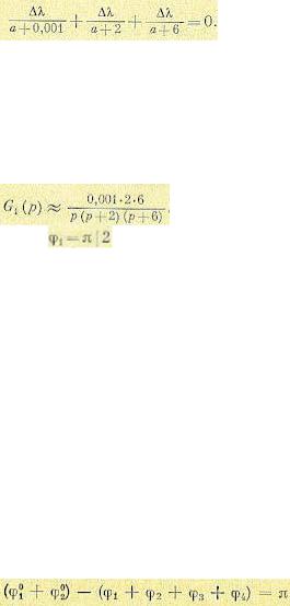
откуда аргумент комплексного числа 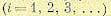и, значит, аргумент числа , т. е. наклон искомых асимптот, будет

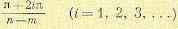(12.41)

3.На вещественной оси траектории корней представляют собой отрезки прямой, соединяющие нули и полюсы функции G (р), расположенные на этой оси. Началом траекторий на вещественной оси служит нуль, расположенный правее всех остальных.

4.Если траектория отклоняется от вещественной оси, то положение точки р = а, в которой траектория отходит от этой оси, можно оценить из того условия, что при малом отклонении , от вещественной оси приращение угла (12.35), обусловленное влиянием полюсов и нулей функции G (р), расположенных на оси влево от искомой точки, должно уничтожаться приращением этого же угла, обусловленным влиянием полюсов и нулей О (р), расположенных вправо от этой точки.

Так, например, пусть имеется функция

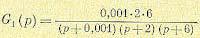(12.42)

При К = 0 траектории исходят из точек (—0,001), (—2) и (—6), лежащих на вещественной

оси. Отрезки траекторий лежат между точками (—0,001) ж (—2) и между (—6) и . Применяя правило 4, можем записать

Решение этого квадратного уравнения дает .

5. Положение точки, в которой траектория пересекает мнимую ось при переходе в правую полуплоскость комплексной переменной р, часто можно оценить, пренебрегая влиянием малого по абсолютной величине полюса функции G (р).

Рассмотрим в качестве примера опять функцию (12.42). При значительных по модулю величинах комплексной переменной р эту функцию можно с хорошей точностью аппроксимировать функцией

Тогда (рис. 12.2) и, следовательно, условие (12.38) сводится к равенству

и Рассматривая график на рис. 12.2, можно заметить, что

откуда следует, что . Это равенство и представляет собой условие для определения точки пересечения В.

6. Направление касательной к траектории при выходе ее из какого-либо полюса или при подходе к какому-либо нулю нетрудно определить путем вычисления угла между этой касательной в данном полюсе или нуле и вещественной осью. При таком вычислении используется зависимость (12.38) для аргументов всех нулей и полюсов, расположенных по условию в левой полуплоскости комплексной переменной р.

На рис. 12.3 изображены траектории корней передаточной функции G (р), имеющей два нуля и два полюса на вещественной оси и одну пару комплексных сопряженных полюсов. При

достаточно малом удалении точки р от полюса q4 углы , соответствующие

остальным нулям и полюсам, останутся неизменными. Таким образом, в силу (12.38) угол найдется из уравнения I

From Wikipedia, the free encyclopedia

The MSE is a measure of the quality of an estimator. As it is derived from the square of Euclidean distance, it is always a positive value that decreases as the error approaches zero.

Definition and basic properties[edit]

Predictor[edit]

${displaystyle operatorname {MSE} ={frac {1}{n}}sum _{i=1}^{n}left(Y_{i}-{hat {Y_{i}}}right)^{2}.}$

In matrix notation,

${displaystyle operatorname {MSE} ={frac {1}{n}}sum _{i=1}^{n}(e_{i})^{2}={frac {1}{n}}mathbf {e} ^{mathsf {T}}mathbf {e} }$

where $e_{i}$ is ${displaystyle (Y_{i}-{hat {Y_{i}}})}$ and is the column vector.

${displaystyle operatorname {MSE} ={frac {1}{q}}sum _{i=n+1}^{n+q}left(Y_{i}-{hat {Y_{i}}}right)^{2}.}$

Estimator[edit]

The MSE of an estimator with respect to an unknown parameter theta is defined as^[1]

${displaystyle operatorname {MSE} ({hat {theta }})=operatorname {E} _{theta }left[({hat {theta }}-theta )^{2}right].}$

${displaystyle operatorname {MSE} ({hat {theta }})=operatorname {Var} _{theta }({hat {theta }})+operatorname {Bias} ({hat {theta }},theta )^{2}.}$

Proof of variance and bias relationship[edit]

In regression[edit]

Examples[edit]

Mean[edit]

$overline{X}=frac{1}{n}sum_{i=1}^n X_i$

which has an expected value equal to the true mean (so it is unbiased) and a mean squared error of

${displaystyle operatorname {MSE} left({overline {X}}right)=operatorname {E} left[left({overline {X}}-mu right)^{2}right]=left({frac {sigma }{sqrt {n}}}right)^{2}={frac {sigma ^{2}}{n}}}$

where $sigma ^{2}$ is the population variance.

For a Gaussian distribution, this is the best unbiased estimator (i.e., one with the lowest MSE among all unbiased estimators), but not, say, for a uniform distribution.

Variance[edit]

The usual estimator for the variance is the corrected sample variance:

${displaystyle S_{n-1}^{2}={frac {1}{n-1}}sum _{i=1}^{n}left(X_{i}-{overline {X}}right)^{2}={frac {1}{n-1}}left(sum _{i=1}^{n}X_{i}^{2}-n{overline {X}}^{2}right).}$

This is unbiased (its expected value is $sigma ^{2}$ ), hence also called the unbiased sample variance, and its MSE is^[8]

${displaystyle operatorname {MSE} (S_{n-1}^{2})={frac {1}{n}}left(mu _{4}-{frac {n-3}{n-1}}sigma ^{4}right)={frac {1}{n}}left(gamma _{2}+{frac {2n}{n-1}}right)sigma ^{4},}$

where $mu _{4}$ is the fourth central moment of the distribution or population, and is the excess kurtosis.

However, one can use other estimators for $sigma ^{2}$ which are proportional to $S^2_{n-1}$ , and an appropriate choice can always give a lower mean squared error. If we define

${displaystyle S_{a}^{2}={frac {n-1}{a}}S_{n-1}^{2}={frac {1}{a}}sum _{i=1}^{n}left(X_{i}-{overline {X}},right)^{2}}$

then we calculate:

This is minimized when

$a=frac{(n-1)gamma_2+n^2+n}{n} = n+1+frac{n-1}{n}gamma_2.$

Gaussian distribution[edit]

The following table gives several estimators of the true parameters of the population, μ and σ², for the Gaussian case.^[9]

True value	Estimator	Mean squared error
	= the unbiased estimator of the population mean, $overline{X}=frac{1}{n}sum_{i=1}^n(X_i)$	$operatorname{MSE}(overline{X})=operatorname{E}((overline{X}-mu)^2)=left(frac{sigma}{sqrt{n}}right)^2$
${displaystyle theta =sigma ^{2}}$	= the unbiased estimator of the population variance, $S^2_{n-1} = frac{1}{n-1}sum_{i=1}^nleft(X_i-overline{X},right)^2$	$operatorname{MSE}(S^2_{n-1})=operatorname{E}((S^2_{n-1}-sigma^2)^2)=frac{2}{n - 1}sigma^4$
${displaystyle theta =sigma ^{2}}$	= the biased estimator of the population variance, $S^2_{n} = frac{1}{n}sum_{i=1}^nleft(X_i-overline{X},right)^2$	$operatorname{MSE}(S^2_{n})=operatorname{E}((S^2_{n}-sigma^2)^2)=frac{2n - 1}{n^2}sigma^4$
${displaystyle theta =sigma ^{2}}$	= the biased estimator of the population variance, $S^2_{n+1} = frac{1}{n+1}sum_{i=1}^nleft(X_i-overline{X},right)^2$	$operatorname{MSE}(S^2_{n+1})=operatorname{E}((S^2_{n+1}-sigma^2)^2)=frac{2}{n + 1}sigma^4$

Interpretation[edit]

An MSE of zero, meaning that the estimator predicts observations of the parameter theta with perfect accuracy, is ideal (but typically not possible).

MSE is also used in several stepwise regression techniques as part of the determination as to how many predictors from a candidate set to include in a model for a given set of observations.

Applications[edit]

Minimizing MSE is a key criterion in selecting estimators: see minimum mean-square error. Among unbiased estimators, minimizing the MSE is equivalent to minimizing the variance, and the estimator that does this is the minimum variance unbiased estimator. However, a biased estimator may have lower MSE; see estimator bias.
In statistical modelling the MSE can represent the difference between the actual observations and the observation values predicted by the model. In this context, it is used to determine the extent to which the model fits the data as well as whether removing some explanatory variables is possible without significantly harming the model’s predictive ability.
In forecasting and prediction, the Brier score is a measure of forecast skill based on MSE.

Loss function[edit]

Criticism[edit]

Notes[edit]

^ This can be proved by Jensen’s inequality as follows. The fourth central moment is an upper bound for the square of variance, so that the least value for their ratio is one, therefore, the least value for the excess kurtosis is −2, achieved, for instance, by a Bernoulli with p=1/2.

References[edit]

^ ^a ^b «Mean Squared Error (MSE)». www.probabilitycourse.com. Retrieved 2020-09-12.
^ Bickel, Peter J.; Doksum, Kjell A. (2015). Mathematical Statistics: Basic Ideas and Selected Topics. Vol. I (Second ed.). p. 20. If we use quadratic loss, our risk function is called the mean squared error (MSE) …
^ ^a ^b Lehmann, E. L.; Casella, George (1998). Theory of Point Estimation (2nd ed.). New York: Springer. ISBN 978-0-387-98502-2. MR 1639875.
^ Gareth, James; Witten, Daniela; Hastie, Trevor; Tibshirani, Rob (2021). An Introduction to Statistical Learning: with Applications in R. Springer. ISBN 978-1071614174.
^ Wackerly, Dennis; Mendenhall, William; Scheaffer, Richard L. (2008). Mathematical Statistics with Applications (7 ed.). Belmont, CA, USA: Thomson Higher Education. ISBN 978-0-495-38508-0.
^ A modern introduction to probability and statistics : understanding why and how. Dekking, Michel, 1946-. London: Springer. 2005. ISBN 978-1-85233-896-1. OCLC 262680588.{{cite book}}: CS1 maint: others (link)
^ Steel, R.G.D, and Torrie, J. H., Principles and Procedures of Statistics with Special Reference to the Biological Sciences., McGraw Hill, 1960, page 288.
^ Mood, A.; Graybill, F.; Boes, D. (1974). Introduction to the Theory of Statistics (3rd ed.). McGraw-Hill. p. 229.
^ DeGroot, Morris H. (1980). Probability and Statistics (2nd ed.). Addison-Wesley.
^ Berger, James O. (1985). «2.4.2 Certain Standard Loss Functions». Statistical Decision Theory and Bayesian Analysis (2nd ed.). New York: Springer-Verlag. p. 60. ISBN 978-0-387-96098-2. MR 0804611.
^ Bermejo, Sergio; Cabestany, Joan (2001). «Oriented principal component analysis for large margin classifiers». Neural Networks. 14 (10): 1447–1461. doi:10.1016/S0893-6080(01)00106-X. PMID 11771723.

Применим закон распределения равновероятности:

(4)

Подставляя (1) и (2) и (4) и вводя обозначения с фазой

Последовательная схема может быть
также реализована на основе СФ.

Нормальные
и аномальные ошибки.

Необходимо рассматривать

,
тогда

если ,
либо соответствует , то

Статистические
критерии оценки непрерывных параметров

сигнала.

Cуществуют
следующие критерии:

ü
Критерий максимума функции правдоподобия.

ü
максимальная апостериорная плотность распределения вероятности
параметра .

ü
Критерий минимума средне квадратичной ошибки.

ü
Критерий Баеса.

Распишем каждый критерий более
подробно.

Критерий максимального
правдоподобия.

оценка
максимального правдоподобия.

Критерий максимальной
апостериорной вероятности.

Рассмотрим статистическую схему:

Оценивается значение
максимального параметра.

Критерий минимальной средне
квадратичной ошибки.

Шумовая составляющая:

Дисперсия:

При проектировании задают
соотношение сигнал/шум, чтобы избежать аномальных ошибок.

А среднеквадратичная ошибка
параметра .

Расчёт среднеквадратической ошибки.

Рассмотрим формулу исходя из
геометрического происхождения сигнала.

Источник

Задача оптимизации
формируется следующим образом.

Имеется система
автоматического управления заданной
структуры. Необходимо так выбрать
параметры этой системы, чтобы получить
минимум среднеквадратичной ошибки при
заданных статистических характеристиках
полезного сигнала и помехи.

Обозначим

–
выходной сигнал системы, оптимальной
по критерию минимума среднеквадратичной
ошибки.

Если

–
выходной сигнал любой другой системы
данного класса (неоптимальной), то

, (4.5)

где

–
требуемый выходной сигнал (аргумент

для простоты записи опущен).

Добавляя

в
скобки правой части неравенства (4.5),
получим

. (4.6)

Следовательно, из
(4.5) и (4.6):

, (4.7)

где

. (4.7)

Из равенства (4.7)
следует, что для выполнения неравенства
(4.5) необходимо, чтобы

(4.8)

. (4.9)

Так как первое
слагаемое в правой части равенства
(4.7) всегда положительно, то для выполнения
требования (4.8) достаточно приравнять
нулю второе слагаемое равенства (4.7):

. (4.10)

Требование (4.9) по
физическому смыслу говорит о том, что
величина среднеквадратичной ошибки
оптимальной системы всегда конечна.
Формально это значит, что в состав
сигнала

не
должен входить белый шум.

Равенство (4.10)
вместе с ограничением по виду выходного
сигнала оптимальной системы является
общим
условием минимума
среднеквадратичной ошибки.

26. Уравнение оптимальной линейной системы.

Получим уравнение,
определяющее оптимальную линейную
систему.

Примем за динамическую
характеристику линейной оптимальной
системы весовую функцию

.

Выходной сигнал
оптимальной системы определяется
формулой

(4.11)

где

–
входной сигнал системы;

–
время наблюдения входного сигнала
(здесь и далее полагается

).

Весовую функцию
произвольной линейной системы представим
в виде

. (4.12)

Тогда сигнал на
выходе произвольной системы будет равен

. (4.13)

Критерием
оптимальности данной системы будем
считать минимум среднеквадратичной
ошибки.

В соответствии с
полученным условием (4.10) с учётом (4.13)
запишем

. (4.14)

После умножения
выражения в круглых скобках на

и выполнения операции математического
ожидания получаем

,

(4.15)

где обозначено

. (4.16)

В общем случае,
когда

и функция

,
равенство (4.15) будет удовлетворяться
при условии, что равно нулю выражение
в скобках, т.е.

. (4.17)

Выражение (4.17) и
есть уравнение, определяющее оптимальную
линейную систему. Оно называется
интегральным уравнением Винера-Хонфа
и получено из условия (4.10).

Определение весовой функции оптимальной линейной системы

Предполагается,
что мы умеем найти

– весовую функцию системы, преобразующую
данную случайную функцию X(t)
в белый шум V(t).

При этом известна
весовая функция обратной системы

,
формирующей X(t)
из белого шума V(t),
т.е.

(4.28)

Обозначим весовую
функцию оптимальной линейной системы
для белого шума V(t)
на входе
через

.

Искомая оптимальная
система представляет собой последовательное
соединение линейных систем с весовыми
функциями

(рис 4.2).

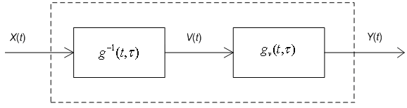
Рис. 4.2. Оптимальная
система

Ранее была получена
формула для

, (4.29)

где

–
интенсивность белого шума V(t).

По формуле для
последовательного соединения систем,
описываемых весовыми функциями, имеем

В данном случае

–
переменная интегрирования

,

–
момент действия на систему —функции
(входного сигнала).

Существуют
аналитические методы решения задачи,
когда функция X(t)
стационарна и имеет дробно-рациональную
спектральную плотность.

Соседние файлы в предмете [НЕСОРТИРОВАННОЕ]

Источник

Критерий — минимум — среднеквадратичная ошибка

Cтраница 1

Идея приближения по критерию минимума среднеквадратичной ошибки, как уже указывалось, не единственна.
[2]

Первое из этих условий удовлетворялось и при синтезе по критерию минимума среднеквадратичной ошибки.
[4]

Страницы:

Источник

Motivation[edit]

Definition[edit]

Properties[edit]

Linear MMSE estimator[edit]

Univariate case[edit]

Computation[edit]

Linear MMSE estimator for linear observation process[edit]

Alternative form[edit]

Sequential linear MMSE estimation[edit]

Special case: scalar observations[edit]

Examples[edit]

Example 1[edit]

Example 2[edit]

Example 3[edit]

Example 4[edit]

See also[edit]

Notes[edit]

Further reading[edit]

Motivation[edit]

Definition[edit]

Properties[edit]

Linear MMSE estimator[edit]

Univariate case[edit]

Computation[edit]

Linear MMSE estimator for linear observation process[edit]

Alternative form[edit]

Sequential linear MMSE estimation[edit]

Special case: scalar observations[edit]

Examples[edit]

Example 1[edit]

Example 2[edit]

Example 3[edit]

Example 4[edit]

See also[edit]

Notes[edit]

Further reading[edit]

Спектральная плотность вычисляется по известной корреляционной функции при помощи формул.

Лекция 59

Учебный материал Расчеты по минимуму среднеквадратичной ошибки

Критерий — минимум — среднеквадратичная ошибка

Definition and basic properties[edit]

Predictor[edit]

Estimator[edit]

Proof of variance and bias relationship[edit]

In regression[edit]

Examples[edit]

Mean[edit]

Variance[edit]

Gaussian distribution[edit]

Interpretation[edit]

Applications[edit]

Loss function[edit]

Criticism[edit]

See also[edit]

Notes[edit]

References[edit]

Спектральная плотность вычисляется по известной корреляционной функции при помощи формул.

Лекция 59

Учебный материал Расчеты по минимуму среднеквадратичной ошибки

Motivation[edit]

Definition[edit]

Properties[edit]

Linear MMSE estimator[edit]

Univariate case[edit]

Computation[edit]

Linear MMSE estimator for linear observation process[edit]

Alternative form[edit]

Sequential linear MMSE estimation[edit]

Special case: scalar observations[edit]

[edit]

Examples[edit]

Example 1[edit]

Example 2[edit]

Example 3[edit]

Example 4[edit]

See also[edit]

Notes[edit]

Further reading[edit]

Критерий — минимум — среднеквадратичная ошибка

Definition and basic properties[edit]