Как определить вероятность ошибки

Проверка корректности А/Б тестов

Хабр, привет! Сегодня поговорим о том, что такое корректность статистических критериев в контексте А/Б тестирования. Узнаем, как проверить, является критерий корректным или нет. Разберём пример, в котором тест Стьюдента не работает.

Меня зовут Коля, я работаю аналитиком данных в X5 Tech. Мы с Сашей продолжаем писать серию статей по А/Б тестированию, это наша третья статья. Первые две можно посмотреть тут:

• Стратификация. Как разбиение выборки повышает чувствительность A/Б теста

• Бутстреп и А/Б тестирование

Корректный статистический критерий

В А/Б тестировании при проверке гипотез с помощью статистических критериев можно совершить одну из двух ошибок:

• ошибку первого рода – отклонить нулевую гипотезу, когда на самом деле она верна. То есть сказать, что эффект есть, хотя на самом деле его нет;

• ошибку второго рода – не отклонить нулевую гипотезу, когда на самом деле она неверна. То есть сказать, что эффекта нет, хотя на самом деле он есть.

Совсем не ошибаться нельзя. Чтобы получить на 100% достоверные результаты, нужно бесконечно много данных. На практике получить столько данных затруднительно. Если совсем не ошибаться нельзя, то хотелось бы ошибаться не слишком часто и контролировать вероятности ошибок.

В статистике ошибка первого рода считается более важной. Поэтому обычно фиксируют допустимую вероятность ошибки первого рода, а затем пытаются минимизировать вероятность ошибки второго рода.

Предположим, мы решили, что допустимые вероятности ошибок первого и второго рода равны 0.1 и 0.2 соответственно. Будем называть статистический критерий корректным, если его вероятности ошибок первого и второго рода равны допустимым вероятностям ошибок первого и второго рода соответственно.

Как сделать критерий, в котором вероятности ошибок будут равны допустимым вероятностям ошибок?

Вероятность ошибки первого рода по определению равна уровню значимости критерия. Если уровень значимости положить равным допустимой вероятности ошибки первого рода, то вероятность ошибки первого рода должна стать равной допустимой вероятности ошибки первого рода.

Вероятность ошибки второго рода можно подогнать под желаемое значение, меняя размер групп или снижая дисперсию в данных. Чем больше размер групп и чем ниже дисперсия, тем меньше вероятность ошибки второго рода. Для некоторых гипотез есть готовые формулы оценки размера групп, при которых достигаются заданные вероятности ошибок.

Например, формула оценки необходимого размера групп для гипотезы о равенстве средних:

где и – допустимые вероятности ошибок первого и второго рода, – ожидаемый эффект (на сколько изменится среднее), и – стандартные отклонения случайных величин в контрольной и экспериментальной группах.

Проверка корректности

Допустим, мы работаем в онлайн-магазине с доставкой. Хотим исследовать, как новый алгоритм ранжирования товаров на сайте влияет на среднюю выручку с покупателя за неделю. Продолжительность эксперимента – одна неделя. Ожидаемый эффект равен +100 рублей. Допустимая вероятность ошибки первого рода равна 0.1, второго рода – 0.2.

Оценим необходимый размер групп по формуле:

import numpy as np
from scipy import stats

alpha = 0.1                     # допустимая вероятность ошибки I рода
beta = 0.2                      # допустимая вероятность ошибки II рода
mu_control = 2500               # средняя выручка с пользователя в контрольной группе
effect = 100                    # ожидаемый размер эффекта
mu_pilot = mu_control + effect  # средняя выручка с пользователя в экспериментальной группе
std = 800                       # стандартное отклонение

# исторические данные выручки для 10000 клиентов
values = np.random.normal(mu_control, std, 10000)

def estimate_sample_size(effect, std, alpha, beta):
    """Оценка необходимого размер групп."""
    t_alpha = stats.norm.ppf(1 - alpha / 2, loc=0, scale=1)
    t_beta = stats.norm.ppf(1 - beta, loc=0, scale=1)
    var = 2 * std ** 2
    sample_size = int((t_alpha + t_beta) ** 2 * var / (effect ** 2))
    return sample_size

estimated_std = np.std(values)
sample_size = estimate_sample_size(effect, estimated_std, alpha, beta)
print(f'оценка необходимого размера групп = {sample_size}')

оценка необходимого размера групп = 784

Чтобы проверить корректность, нужно знать природу случайных величин, с которыми мы работаем. В этом нам помогут исторические данные. Представьте, что мы перенеслись в прошлое на несколько недель назад и запустили эксперимент с таким же дизайном, как мы планировали запустить его сейчас. Дизайн – это совокупность параметров эксперимента, таких как: целевая метрика, допустимые вероятности ошибок первого и второго рода, размеры групп и продолжительность эксперимента, техники снижения дисперсии и т.д.

Так как это было в прошлом, мы знаем, какие покупки совершили пользователи, можем вычислить метрики и оценить значимость отличий. Кроме того, мы знаем, что эффекта на самом деле не было, так как в то время эксперимент на самом деле не запускался. Если значимые отличия были найдены, то мы совершили ошибку первого рода. Иначе получили правильный результат.

Далее нужно повторить эту процедуру с мысленным запуском эксперимента в прошлом на разных группах и временных интервалах много раз, например, 1000.

После этого можно посчитать долю экспериментов, в которых была совершена ошибка. Это будет точечная оценка вероятности ошибки первого рода.

Оценку вероятности ошибки второго рода можно получить аналогичным способом. Единственное отличие состоит в том, что каждый раз нужно искусственно добавлять ожидаемый эффект в данные экспериментальной группы. В этих экспериментах эффект на самом деле есть, так как мы сами его добавили. Если значимых отличий не будет найдено – это ошибка второго рода. Проведя 1000 экспериментов и посчитав долю ошибок второго рода, получим точечную оценку вероятности ошибки второго рода.

Посмотрим, как оценить вероятности ошибок в коде. С помощью численных синтетических А/А и А/Б экспериментов оценим вероятности ошибок и построим доверительные интервалы:

def run_synthetic_experiments(values, sample_size, effect=0, n_iter=10000):
    """Проводим синтетические эксперименты, возвращаем список p-value."""
    pvalues = []
    for _ in range(n_iter):
        a, b = np.random.choice(values, size=(2, sample_size,), replace=False)
        b += effect
        pvalue = stats.ttest_ind(a, b).pvalue
        pvalues.append(pvalue)
    return np.array(pvalues)

def print_estimated_errors(pvalues_aa, pvalues_ab, alpha):
    """Оценивает вероятности ошибок."""
    estimated_first_type_error = np.mean(pvalues_aa < alpha)
    estimated_second_type_error = np.mean(pvalues_ab >= alpha)
    ci_first = estimate_ci_bernoulli(estimated_first_type_error, len(pvalues_aa))
    ci_second = estimate_ci_bernoulli(estimated_second_type_error, len(pvalues_ab))
    print(f'оценка вероятности ошибки I рода = {estimated_first_type_error:0.4f}')
    print(f'  доверительный интервал = [{ci_first[0]:0.4f}, {ci_first[1]:0.4f}]')
    print(f'оценка вероятности ошибки II рода = {estimated_second_type_error:0.4f}')
    print(f'  доверительный интервал = [{ci_second[0]:0.4f}, {ci_second[1]:0.4f}]')

def estimate_ci_bernoulli(p, n, alpha=0.05):
    """Доверительный интервал для Бернуллиевской случайной величины."""
    t = stats.norm.ppf(1 - alpha / 2, loc=0, scale=1)
    std_n = np.sqrt(p * (1 - p) / n)
    return p - t * std_n, p + t * std_n

pvalues_aa = run_synthetic_experiments(values, sample_size, effect=0)
pvalues_ab = run_synthetic_experiments(values, sample_size, effect=effect)
print_estimated_errors(pvalues_aa, pvalues_ab, alpha)

оценка вероятности ошибки I рода = 0.0991
  доверительный интервал = [0.0932, 0.1050]
оценка вероятности ошибки II рода = 0.1978
  доверительный интервал = [0.1900, 0.2056]

Оценки вероятностей ошибок примерно равны 0.1 и 0.2, как и должно быть. Всё верно, тест Стьюдента на этих данных работает корректно.

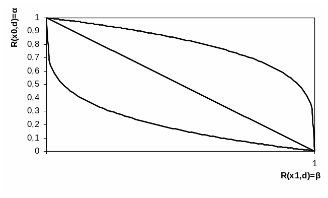
Распределение p-value

Выше рассмотрели случай, когда тест контролирует вероятность ошибки первого рода при фиксированном уровне значимости. Если решим изменить уровень значимости с 0.1 на 0.01, будет ли тест контролировать вероятность ошибки первого рода? Было бы хорошо, если тест контролировал вероятность ошибки первого рода при любом заданном уровне значимости. Формально это можно записать так:

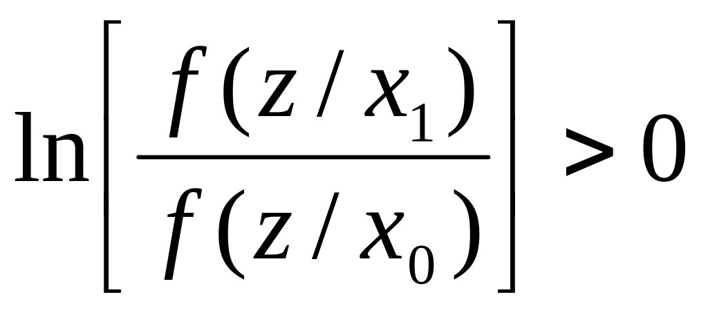
Для любого выполняется .

Заметим, что в левой части равенства записано выражение для функции распределения p-value. Из равенства следует, что функция распределения p-value в точке X равна X для любого X от 0 до 1. Эта функция распределения является функцией распределения равномерного распределения от 0 до 1. Мы только что показали, что статистический критерий контролирует вероятность ошибки первого рода на заданном уровне для любого уровня значимости тогда и только тогда, когда при верности нулевой гипотезы p-value распределено равномерно от 0 до 1.

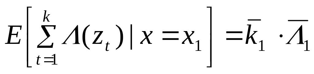
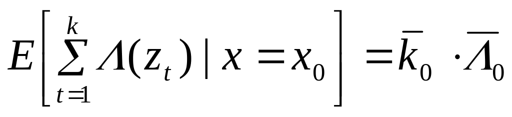
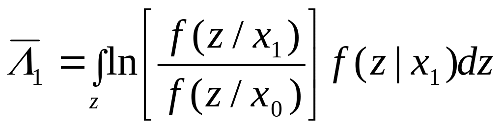
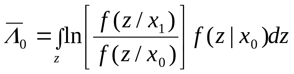
При верности нулевой гипотезы p-value должно быть распределено равномерно. А как должно быть распределено p-value при верности альтернативной гипотезы? Из условия для вероятности ошибки второго рода следует, что .

Получается, график функции распределения p-value при верности альтернативной гипотезы должен проходить через точку , где и – допустимые вероятности ошибок конкретного эксперимента.

Проверим, как распределено p-value в численном эксперименте. Построим эмпирические функции распределения p-value:

import matplotlib.pyplot as plt

def plot_pvalue_distribution(pvalues_aa, pvalues_ab, alpha, beta):
    """Рисует графики распределения p-value."""
    estimated_first_type_error = np.mean(pvalues_aa < alpha)
    estimated_second_type_error = np.mean(pvalues_ab >= alpha)
    y_one = estimated_first_type_error
    y_two = 1 - estimated_second_type_error
    X = np.linspace(0, 1, 1000)
    Y_aa = [np.mean(pvalues_aa < x) for x in X]
    Y_ab = [np.mean(pvalues_ab < x) for x in X]

    plt.plot(X, Y_aa, label='A/A')
    plt.plot(X, Y_ab, label='A/B')
    plt.plot([alpha, alpha], [0, 1], '--k', alpha=0.8)
    plt.plot([0, alpha], [y_one, y_one], '--k', alpha=0.8)
    plt.plot([0, alpha], [y_two, y_two], '--k', alpha=0.8)
    plt.plot([0, 1], [0, 1], '--k', alpha=0.8)

    plt.title('Оценка распределения p-value', size=16)
    plt.xlabel('p-value', size=12)
    plt.legend(fontsize=12)
    plt.grid()
    plt.show()

plot_pvalue_distribution(pvalues_aa, pvalues_ab, alpha, beta)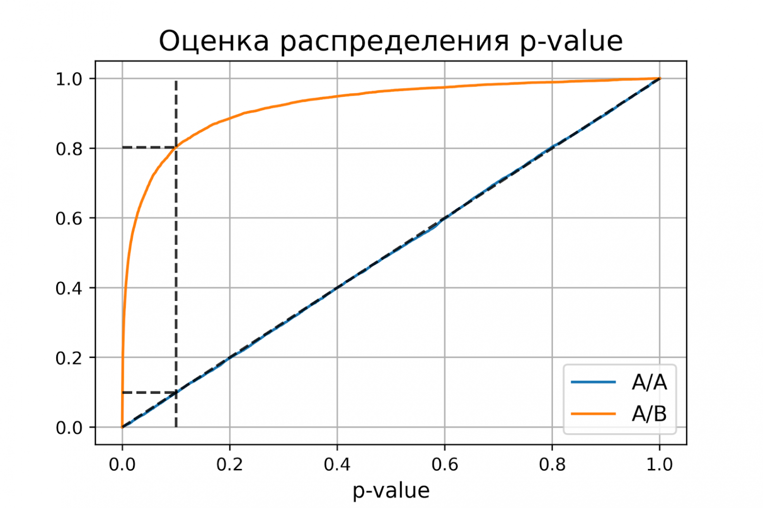

P-value для синтетических А/А тестах действительно оказалось распределено равномерно от 0 до 1, а для синтетических А/Б тестов проходит через точку .

Кроме оценок распределений на графике дополнительно построены четыре пунктирные линии:

• диагональная из точки [0, 0] в точку [1, 1] – это функция распределения равномерного распределения на отрезке от 0 до 1, по ней можно визуально оценивать равномерность распределения p-value;

• вертикальная линия с – пороговое значение p-value, по которому определяем отвергать нулевую гипотезу или нет. Проекция на ось ординат точки пересечения вертикальной линии с функцией распределения p-value для А/А тестов – это вероятность ошибки первого рода. Проекция точки пересечения вертикальной линии с функцией распределения p-value для А/Б тестов – это мощность теста (мощность = 1 — ). 

• две горизонтальные линии – проекции на ось ординат точки пересечения вертикальной линии с функцией распределения p-value для А/А и А/Б тестов.

График с оценками распределения p-value для синтетических А/А и А/Б тестов позволяет проверить корректность теста для любого значения уровня значимости.

Некорректный критерий

Выше рассмотрели пример, когда тест Стьюдента оказался корректным критерием для случайных данных из нормального распределения. Может быть, все критерии всегда работаю корректно, и нет смысла каждый раз проверять вероятности ошибок?

Покажем, что это не так. Немного изменим рассмотренный ранее пример, чтобы продемонстрировать некорректную работу критерия. Допустим, мы решили увеличить продолжительность эксперимента до 2-х недель. Для каждого пользователя будем вычислять стоимость покупок за первую неделю и стоимость покупок за второю неделю. Полученные стоимости будем передавать в тест Стьюдента для проверки значимости отличий. Положим, что поведение пользователей повторяется от недели к неделе, и стоимости покупок одного пользователя совпадают.

def run_synthetic_experiments_two(values, sample_size, effect=0, n_iter=10000):
    """Проводим синтетические эксперименты на двух неделях."""
    pvalues = []
    for _ in range(n_iter):
        a, b = np.random.choice(values, size=(2, sample_size,), replace=False)
        b += effect
        # дублируем данные
        a = np.hstack((a, a,))
        b = np.hstack((b, b,))
        pvalue = stats.ttest_ind(a, b).pvalue
        pvalues.append(pvalue)
    return np.array(pvalues)

pvalues_aa = run_synthetic_experiments_two(values, sample_size)
pvalues_ab = run_synthetic_experiments_two(values, sample_size, effect=effect)
print_estimated_errors(pvalues_aa, pvalues_ab, alpha)
plot_pvalue_distribution(pvalues_aa, pvalues_ab, alpha, beta)

оценка вероятности ошибки I рода = 0.2451
  доверительный интервал = [0.2367, 0.2535]
оценка вероятности ошибки II рода = 0.0894
  доверительный интервал = [0.0838, 0.0950]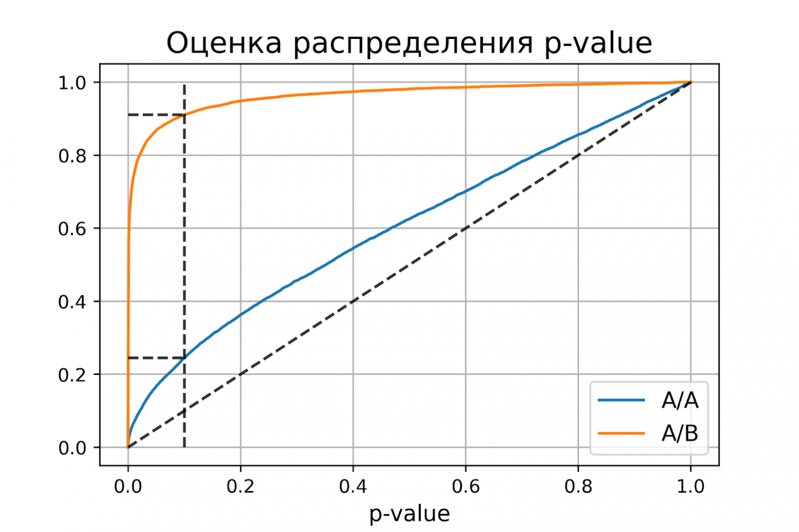

Получили оценку вероятности ошибки первого рода около 0.25, что сильно больше уровня значимости 0.1. На графике видно, что распределение p-value для синтетических А/А тестов не равномерно, оно отклоняется от диагонали. В этом примере тест Стьюдента работает некорректно, так как данные зависимые (стоимости покупок одного человека зависимы). Если бы мы сразу не догадались про зависимость данных, то оценка вероятностей ошибок помогла бы нам понять, что такой тест некорректен.

Итоги

Мы обсудили, что такое корректность статистического теста, посмотрели, как оценить вероятности ошибок на исторических данных и привели пример некорректной работы критерия.

Таким образом:

• корректный критерий – это критерий, у которого вероятности ошибок первого и второго рода равны допустимым вероятностям ошибок первого и второго рода соответственно;

• чтобы критерий контролировал вероятность ошибки первого рода для любого уровня значимости, необходимо и достаточно, чтобы p-value при верности нулевой гипотезы было распределено равномерно от 0 до 1.

5.6. Вероятность ошибки р

Если следовать подразделению статистики на описательную и аналитическую, то задача аналитической статистики — предоставить методы, с помощью которых можно было бы объективно выяснить,
например, является ли наблюдаемая разница в средних значениях или взаимосвязь (корреляция) выборок случайной или нет.

Например, если сравниваются два средних значения выборок, то можно сформулировать две предварительных гипотезы:

• Гипотеза 0 (нулевая): Наблюдаемые различия между средними значениями выборок находятся в пределах случайных отклонений.

• Гипотеза 1 (альтернативная): Наблюдаемые различия между средними значениями нельзя объяснить случайными отклонениями.

В аналитической статистике разработаны методы вычисления так называемых тестовых (контрольных) величин, которые рассчитываются по определенным формулам на основе данных,
содержащихся в выборках или полученных из них характеристик. Эти тестовые величины соответствуют определенным теоретическим распределениям
(t-pacnpeлелению, F-распределению, распределению X2 и т.д.), которые позволяют вычислить так называемую вероятность ошибки. Это вероятность равна проценту ошибки,
которую можно допустить отвергнув нулевую гипотезу и приняв альтернативную.

Вероятность определяется в математике, как величина, находящаяся в диапазоне от 0 до 1. В практической статистике она также часто выражаются в процентах. Обычно вероятность обозначаются буквой р:

0 < р < 1

Вероятности ошибки, при которой допустимо отвергнуть нулевую гипотезу и принять альтернативную гипотезу, зависит от каждого конкретного случая.
В значительной степени эта вероятность определяется характером исследуемой ситуации. Чем больше требуемая вероятность, с которой надо избежать ошибочного решения,
тем более узкими выбираются границы вероятности ошибки, при которой отвергается нулевая гипотеза, так называемый доверительный интервал вероятности.
Обычно в исследованиях используют 5% вероятность ошибки.

Существует общепринятая терминология, которая относится к доверительным интервалам вероятности:

• Высказывания, имеющие вероятность ошибки р <= 0,05 — называются значимыми.
• Высказывания с вероятностью ошибки р <= 0,01 — очень значимыми,
• А высказывания с вероятностью ошибки р <= 0,001 — максимально значимыми.

В литературе такие ситуации иногда обозначают одной, двумя или тремя звездочками.

Вероятность ошибки	Значимость	Обозначение
р > 0.05	Не значимая	ns
р <= 0.05	Значимая	*
р <= 0.01	Очень значимая	**
р <= 0.001	Максимально значимая	***

В SPSS вероятность ошибки р имеет различные обозначения; звездочки для указания степени значимости применяются лишь в немногих случаях. Обычно в SPSS значение р обозначается Sig. (Significant).

Времена, когда не было компьютеров, пригодных для статистического анализа, давали практикам по крайней мере одно преимущество. Так как все вычисления надо было выполнять вручную,
статистик должен был сначала тщательно обдумать, какие вопросы можно решить с помощью того или иного теста. Кроме того, особое значение придавалось точной формулировке нулевой гипотезы.

Но с помощью компьютера и такой мощной программы, как SPSS, очень легко можно провести множество тестов за очень короткое время. К примеру, если в таблицу сопряженности свести 50 переменных
с другими 20 переменными и выполнить тест X², то получится 1000 результатов проверки значимости или 1000 значений р. Некритический подбор значимых величин может
дать бессмысленный результат, так как уже при граничном уровне значимости р = 0,05 в пяти процентах наблюдений, то есть в 50 возможных наблюдениях, можно ожидать значимые результаты.

Этим ошибкам первого рода (когда нулевая гипотеза отвергается, хотя она верна) следует уделять достаточно внимания. Ошибкой второго рода называется ситуация,
когда нулевая гипотеза принимается, хотя она ложна. Вероятность допустить ошибку первого рода равна вероятности ошибки р. Вероятность ошибки второго рода тем меньше, чем больше вероятность ошибки р.

Вероятности ошибок

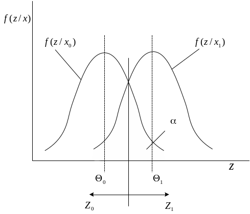
Под ошибкой первого рода понимается
ложная тревога. Вероятность ошибки
первого рода вычисляется как:

— для непрерывной случайной величины

;

— для дискретной случайной величины

.

Под ошибкой второго рода понимается
пропуск цели. Вероятность ошибки второго
рода вычисляется как:

— для непрерывной случайной величины

;

— для дискретной случайной величины

.

Вероятность

– носит название вероятности правильного
обнаружения.

Как правило, наблюдения распределены
по нормальному закону:

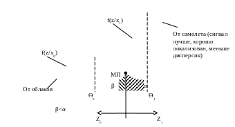
На рисунке ниже показаны ошибки первого
и второго рода для случая нормального
распределения наблюдений.

Обычно, в задачах обнаружения пропуск
цели штрафуется дороже, чем ложная
тревога. Для значений функции потерь,
приведенных в таблице,

,

.

Таблица 1

С(x,d)	d=d1	d=d0
x=x1	c11	c10
x=x0	c01	c00

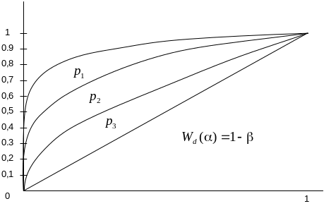
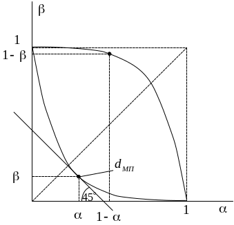
Рабочая характеристика решающего правила

На рисунке ниже показаны характеристики

,

и

семейства решающих правил

.
Характеристика показывает зависимость
вероятности правильного обнаружения
объекта и вероятности ложной тревоги.
Для приведенных характеристик справедливо
следующее соотношение:

.
В качестве примера характеристики
решающего правила можно рассмотрим
отношение сигнал/шум. Тогда, в случае
нормального распределения наблюдений
и при условии, что

,

.

– функция мощности решающего правила.
Под мощностью решающего правила при
заданном значении

понимают вероятность принятия правильного
решения при заданном состоянии среды.

Байесово решающее правило

Условные риски от принятия решающего
правила

равны (здесь и далее используются
значения функции потерь из таблицы 1):

;

.

Средний риск принятия решающего правила

равен:

.

Апостериорный риск принятия решающего
правила

равен:

;

.

Байесовское решающее правило

:

.

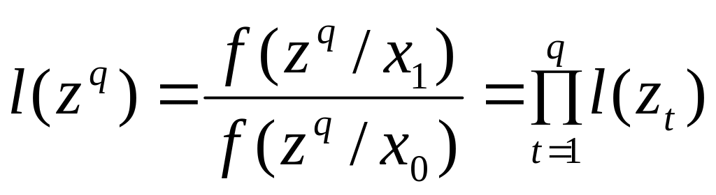
Рассмотрим случай, когда

,
тогда

.

Выполним ряд преобразований:

;

.

С учетом того, что

,
получаем:

.

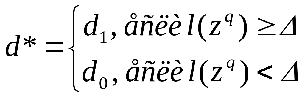
Тогда

,

где

– отношение правдоподобия;

– пороговое значение.

При равных вероятностях

обычно

и тогда

.

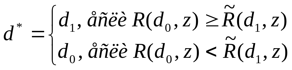
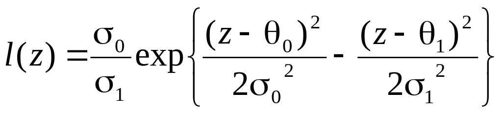
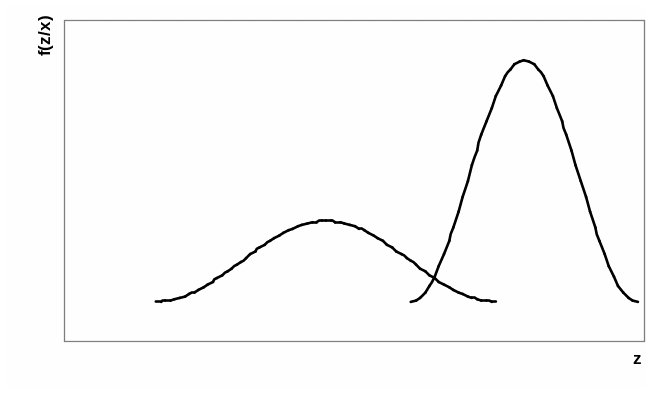
Пример. Пусть задана функция
правдоподобия

,
вероятности нахождения пространства
в различных состояниях одинаковые

,
пороговое значение

.
На рисунке ниже показана функция
правдоподобия и граница разбиения
множества наблюдений

.

Отношение правдоподобия показано на
рис. ниже

Если наблюдения имеют нормальное
распределение, т.е.

;

,
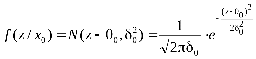
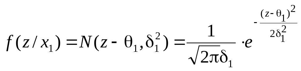
тогда отношение правдоподобия имеет
вид:

.

Для удобства используется логарифм
отношения правдоподобия:

.

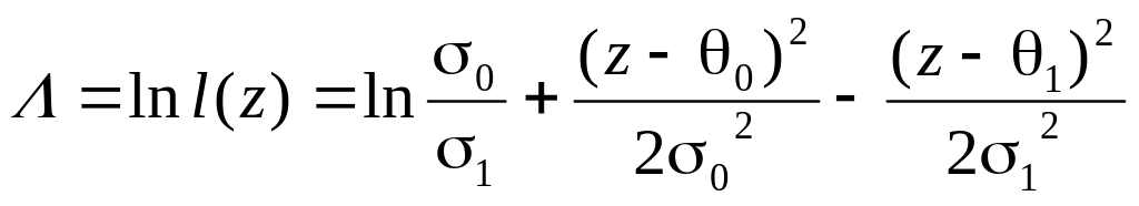
Тогда байесовское решающее правило
имеет вид:

.

Максимум
апостериорной вероятности

Функция потерь

,
где

.
Тогда

,

и пороговое значение

.

Условный риск равен:

;

.

Средний риск равен:

.

Минимизируем вероятность принятия
неправильного решения

Максимум
правдоподобия

При

пороговое значение

.

Средний риск равен:

.

Решающее правило
Неймана-Пирсона

Решающее правило Неймана-Пирсона
представляет собой семейство решающих
правил и является пороговым:

,

где

определяется из условия:

,

где α – заданная вероятность ложной
тревоги.

Решающее правило Неймана-Пирсона принято
характеризовать с использованием
функции мощности решающего правила

.

Лемма Неймана-Пирсона

Решающее правило Неймана-Пирсона для
любого значения вероятности ложной
тревоги и для любого решающего правила
обладает наиболее мощным среди всех
решающих правил:

,

или

,

.

Следствие: Решающее правило
Неймана-Пирсона является допустимым
при простой функции потерь:

— допустимое решающее правило.

Доказательство:

;

и если

,
то

.

Доказательство (леммы):

Пусть

—
пространство наблюдений,

– область пространства наблюдений, при
попадании наблюдения в которую решающее
правило Неймана-Пирсона принимает
значение

,

– область пространства наблюдений, при
попадании наблюдения в которую
произвольное решающее правило принимает
значение

.

Введем ряд обозначений (см. рисунок
ниже):

;

;

.

=

=

При переходе (1) использовалось соотношение:

,

.
При переходе (2) учитывалось, что

,
т.к.

— порог для

,
а

=Ø.

Замечание. При

выполняется строгое равенство

.

Структура решающих
правил

Все решающие правила можно рассматривать
как правила Неймана-Пирсона

при фиксированном с помощью порога
значении

,
а это значит, что и МАВ и МП и байесовские
решающие правила дают допустимую
решающую функцию. В тоже время все
критерии можно рассматривать как
байесовские при постой функции потерь.
В таблице ниже приведены решающие
правила и соответствующие им пороги.

Решающее правило	Порог
Байесово решающее правило
МАВ (максимум апостериорной вероятности)
МП (максимум правдоподобия)	1
Н-П (решающее правило Неймана-Пирсона)	Определяется з условия

Рассмотрим задачу обнаружения самолета
радиолокационными средствами. На рисунке
ниже показаны функции правдоподобия
для состояний среды

и

при наличии наблюдений

.
При отражении сигнала от самолета сигнал
хорошо локализован и имеет меньшую
дисперсию, при отражении от облаков
сигнал плохо локализован.

На рисунках ниже показано множество
решающих правил

и решающие правила для МП, байесова
решающего правила и решающего правила
Неймана-Пирсона.

Решающее правило МП есть точка касания
границы множества

и прямой, проведенной под углом 135° к
оси абсцисс.

Байесово решающее правило есть точка
касания границы множества

и прямой, проходящей через точку

.

Решающее правило Неймана-Пирсона
определяется соответствующими значениями

и

.

d0

Множество точек

обладает свойством поворотной симметрии
относительно прямой

,

,
т.е. симметрией относительно вращения
на 180°. Симметричность области

следует из возможности для любого
разбиения

,

построить разбиение

,

,
тогда

;

.

Асимметрия области относительно
биссектрисы объясняется различием
функций правдоподобия

и

.

Последовательные
решения

До сих пор рассматривалась задача
принятия решения на основе анализа всех
имеющихся измерений (наблюдений). Однако,
если вектор наблюдения

можно рассматривать как последовательность
векторов

,
каждый из которых получен в момент
времени

имеет смысл рассматривать задачу
принятия решения как совокупность двух
задач:

а) принятие решения об остановке
наблюдений;

б) принятия решения по имеющимся к
моменту остановки наблюдения измерениям.

Рассмотрим простую двухальтернативную
задач. Пусть покупателю нужно принять
решение о закупке партии товара, например,
лампочек на основе закупки и исследования
пробной партии. Множество состояний
партии лампочек

,
где

— партия лампочек не является бракованной,

— партия лампочек бракованная. Множество
решений

,
где

— решение о закупке партии лампочек,

— решение об отказе о закупке партии
лампочек. Множество измерений на момент
времени

будем обозначать

,

.
Пусть измерения являются независимыми:

.
Требуется определить момент

,
после которого наблюдения дальше не
производятся и по совокупности измерений

принять решение

или

.

Рассмотрим разбиение пространства

,
где

— область продолжения наблюдений,

— область принятия решения

,

— область принятия решения

.
При этом

Ø,

.

В качестве критерия оптимальности будем
использовать среднее количество
измерений

,
необходимое для принятия решения при
заданных вероятностях ошибок I
и II рода.

Для принятия решения будем использовать
отношение правдоподобия

,

или его логарифм

,

.

Математик А. Вальд (1947 г.) показал, что
при заданных ошибках первого рода

и второго рода

наименьшим временем анализа обладает
процедура вида:

,

где

и

— некоторые пороговые значения.

На рисунке ниже показаны пороги

и

на пря мой

.

Покажем, что для порогов

и

справедливы следующие соотношения:

,

.

Действительно,

,
где при переходе (1) учтено, что

,

.

Аналогично:


,
где при переходе (1) учтено, что,

,

.

На рисунке ниже показаны пороги

и

на пря мой

с учетом полученных соотношений.

Замечание. Для того чтобы обеспечить
выполнение неравенства

достаточно, что бы

,

.
Действительно,

,
тогда

.
Из получено неравенства следует, что

и

.

Точные значения порогов вычислить
трудно, поэтому полагают, что:

,

.
Тогда решения становятся более осторожными
и увеличивается среднее время до принятия
решения, т.е. в рассматриваемом примере
увеличивается количество лампочек,
которые нужно проверить до принятия
решения.

При изменении пороговых значений
вероятности ошибок I и II
рода также изменятся:

,

.
Для новых значений вероятностей
выполняются следующие соотношения:

,
откуда

.

Сложив неравенства, получаем:

;

,

откуда

.

Примечание. На практике обычно
работают с логарифмом отношения
правдоподобия

.
Тогда

;

;

.

При работе с логарифмом отношения
правдоподобия для нормального закона
не требуется вычислять экспоненту.

На рисунке ниже показаны пороги

и

на пря мой

.

Утверждение. Количество наблюдений

до остановки наблюдений конечно, т.е.
процедура последовательного анализа
является конечной:

,
как при принятии решения

,
так и при принятии решения

.

Лемма. Пусть

– последовательность независимых
одинаково распределенных случайных
величин с математическим ожиданием

случайных величин. Тогда для всякой
последовательной процедуры со свойством

имеет место равенство:

.

Оценка количества
наблюдений

Пусть множество состояний природы

,
множество решений

.
Рассмотрим две гипотезы:

,

.

При состоянии природы

получаем

,
где

,
где

— номер последнего наблюдения, где

,

.

При состоянии природы

получаем

,
где

,
где

— номер последнего наблюдения, где

.

.

В среднем для принятия решения

необходимо выполнить

измерений, для принятия решения

необходимо в среднем

измерений.

На рисунке ниже показаны функции
апостериорной вероятности для состояний
среды

и

при наличии наблюдения

.

Значения

,

.

Если

,
тогда

.
Если

,
тогда

,
и принимается решение

.

В общем виде для принятия некоторого
решения

необходимо в среднем выполнить

измерений:

,

.

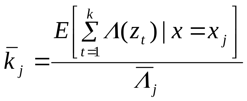
Найдем числитель этого выражения. Для
этого будем считать, что в момент
остановки

или

.

Тогда вероятности событий равны:

Откуда

,
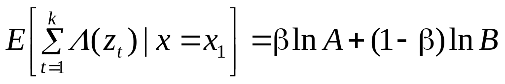
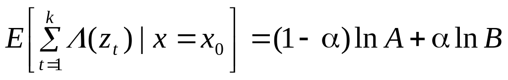
тогда

,

.

Усеченные процедуры

Последовательная процедура имеет
минимальное среднее время анализа,
однако некоторая реализация процедуры
может оказаться непомерно длинной.
Поэтому, обычно, заранее выбирают число

,
являющееся максимальным номером
наблюдения, исходя из заданной вероятности

.
Если решение не принято последовательной
процедурой, то оно принимается, например,
по методу Неймана-Пирсона. При этом
ухудшается качество решения, т.е.

оказывается больше.

Пусть провели серию из

наблюдений. В результате был получен
вектор наблюдений

.
После

наблюдений ресурс наблюдений оказался
исчерпан. Применим классическую схему:
вычислим отношение правдоподобия

,
решение

,
где ∆ – пороговое значение.

Усеченная пороговая процедура дает
решения хуже по сравнению с классической
процедурой, поскольку при принятии
решения используется аномальная
последовательность наблюдений.

Наблюдение в форме
прогноза

Соседние файлы в предмете [НЕСОРТИРОВАННОЕ]

• #
• #
• #
• #
• #
• #
• #
• #
• #
• #
• #

This article is about erroneous outcomes of statistical tests. For closely related concepts in binary classification and testing generally, see false positives and false negatives.

In statistical hypothesis testing, a type I error is the mistaken rejection of a null hypothesis that is actually true. A type I error is also known as a «false positive» finding or conclusion; example: «an innocent person is convicted». A type II error is the failure to reject a null hypothesis that is actually false. A type II error is also known as a «false negative» finding or conclusion; example: «a guilty person is not convicted».^[1] Much of statistical theory revolves around the minimization of one or both of these errors, though the complete elimination of either is a statistical impossibility if the outcome is not determined by a known, observable causal process.
By selecting a low threshold (cut-off) value and modifying the alpha (α) level, the quality of the hypothesis test can be increased.^{[citation needed]} The knowledge of type I errors and type II errors is widely used in medical science, biometrics and computer science.^{[clarification needed]}

Intuitively, type I errors can be thought of as errors of commission (i.e., the researcher unluckily concludes that something is the fact). For instance, consider a study where researchers compare a drug with a placebo. If the patients who are given the drug get better than the patients given the placebo by chance, it may appear that the drug is effective, but in fact the conclusion is incorrect.
In reverse, type II errors are errors of omission. In the example above, if the patients who got the drug did not get better at a higher rate than the ones who got the placebo, but this was a random fluke, that would be a type II error. The consequence of a type II error depends on the size and direction of the missed determination and the circumstances. An expensive cure for one in a million patients may be inconsequential even if it truly is a cure.

Definition[edit]

Statistical background[edit]

In statistical test theory, the notion of a statistical error is an integral part of hypothesis testing. The test goes about choosing about two competing propositions called null hypothesis, denoted by H₀ and alternative hypothesis, denoted by H₁. This is conceptually similar to the judgement in a court trial. The null hypothesis corresponds to the position of the defendant: just as he is presumed to be innocent until proven guilty, so is the null hypothesis presumed to be true until the data provide convincing evidence against it. The alternative hypothesis corresponds to the position against the defendant. Specifically, the null hypothesis also involves the absence of a difference or the absence of an association. Thus, the null hypothesis can never be that there is a difference or an association.

If the result of the test corresponds with reality, then a correct decision has been made. However, if the result of the test does not correspond with reality, then an error has occurred. There are two situations in which the decision is wrong. The null hypothesis may be true, whereas we reject H₀. On the other hand, the alternative hypothesis H₁ may be true, whereas we do not reject H₀. Two types of error are distinguished: type I error and type II error.^[2]

Type I error[edit]

The first kind of error is the mistaken rejection of a null hypothesis as the result of a test procedure. This kind of error is called a type I error (false positive) and is sometimes called an error of the first kind. In terms of the courtroom example, a type I error corresponds to convicting an innocent defendant.

Type II error[edit]

The second kind of error is the mistaken failure to reject the null hypothesis as the result of a test procedure. This sort of error is called a type II error (false negative) and is also referred to as an error of the second kind. In terms of the courtroom example, a type II error corresponds to acquitting a criminal.^[3]

Crossover error rate[edit]

The crossover error rate (CER) is the point at which type I errors and type II errors are equal. A system with a lower CER value provides more accuracy than a system with a higher CER value.

False positive and false negative[edit]

In terms of false positives and false negatives, a positive result corresponds to rejecting the null hypothesis, while a negative result corresponds to failing to reject the null hypothesis; «false» means the conclusion drawn is incorrect. Thus, a type I error is equivalent to a false positive, and a type II error is equivalent to a false negative.

Table of error types[edit]

Tabularised relations between truth/falseness of the null hypothesis and outcomes of the test:^[4]

Table of error types	Null hypothesis (H0) is
True	False
Decision about null hypothesis (H0)	Fail to reject	Correct inference (true negative) (probability = 1−α)	Type II error (false negative) (probability = β)
Reject	Type I error (false positive) (probability = α)	Correct inference (true positive) (probability = 1−β)

Error rate[edit]

A perfect test would have zero false positives and zero false negatives. However, statistical methods are probabilistic, and it cannot be known for certain whether statistical conclusions are correct. Whenever there is uncertainty, there is the possibility of making an error. Considering this nature of statistics science, all statistical hypothesis tests have a probability of making type I and type II errors.^{[citation needed]}

• The type I error rate is the probability of rejecting the null hypothesis given that it is true. The test is designed to keep the type I error rate below a prespecified bound called the significance level, usually denoted by the Greek letter α (alpha) and is also called the alpha level. Usually, the significance level is set to 0.05 (5%), implying that it is acceptable to have a 5% probability of incorrectly rejecting the true null hypothesis.^[5]
• The rate of the type II error is denoted by the Greek letter β (beta) and related to the power of a test, which equals 1−β.^{[citation needed]}

These two types of error rates are traded off against each other: for any given sample set, the effort to reduce one type of error generally results in increasing the other type of error.^{[citation needed]}

The quality of hypothesis test[edit]

The same idea can be expressed in terms of the rate of correct results and therefore used to minimize error rates and improve the quality of hypothesis test. To reduce the probability of committing a type I error, making the alpha value more stringent is quite simple and efficient. To decrease the probability of committing a type II error, which is closely associated with analyses’ power, either increasing the test’s sample size or relaxing the alpha level could increase the analyses’ power.^{[citation needed]} A test statistic is robust if the type I error rate is controlled.

Varying different threshold (cut-off) value could also be used to make the test either more specific or more sensitive, which in turn elevates the test quality. For example, imagine a medical test, in which an experimenter might measure the concentration of a certain protein in the blood sample. The experimenter could adjust the threshold (black vertical line in the figure) and people would be diagnosed as having diseases if any number is detected above this certain threshold. According to the image, changing the threshold would result in changes in false positives and false negatives, corresponding to movement on the curve.^{[citation needed]}

Example[edit]

Since in a real experiment it is impossible to avoid all type I and type II errors, it is important to consider the amount of risk one is willing to take to falsely reject H₀ or accept H₀. The solution to this question would be to report the p-value or significance level α of the statistic. For example, if the p-value of a test statistic result is estimated at 0.0596, then there is a probability of 5.96% that we falsely reject H₀. Or, if we say, the statistic is performed at level α, like 0.05, then we allow to falsely reject H₀ at 5%. A significance level α of 0.05 is relatively common, but there is no general rule that fits all scenarios.

Vehicle speed measuring[edit]

The speed limit of a freeway in the United States is 120 kilometers per hour (75 mph). A device is set to measure the speed of passing vehicles. Suppose that the device will conduct three measurements of the speed of a passing vehicle, recording as a random sample X₁, X₂, X₃. The traffic police will or will not fine the drivers depending on the average speed . That is to say, the test statistic

In addition, we suppose that the measurements X₁, X₂, X₃ are modeled as normal distribution N(μ,4). Then, T should follow N(μ,4/3) and the parameter μ represents the true speed of passing vehicle. In this experiment, the null hypothesis H₀ and the alternative hypothesis H₁ should be

H₀: μ=120     against      H₁: μ>120.

If we perform the statistic level at α=0.05, then a critical value c should be calculated to solve

According to change-of-units rule for the normal distribution. Referring to Z-table, we can get

Here, the critical region. That is to say, if the recorded speed of a vehicle is greater than critical value 121.9, the driver will be fined. However, there are still 5% of the drivers are falsely fined since the recorded average speed is greater than 121.9 but the true speed does not pass 120, which we say, a type I error.

The type II error corresponds to the case that the true speed of a vehicle is over 120 kilometers per hour but the driver is not fined. For example, if the true speed of a vehicle μ=125, the probability that the driver is not fined can be calculated as

which means, if the true speed of a vehicle is 125, the driver has the probability of 0.36% to avoid the fine when the statistic is performed at level α=0.05, since the recorded average speed is lower than 121.9. If the true speed is closer to 121.9 than 125, then the probability of avoiding the fine will also be higher.

The tradeoffs between type I error and type II error should also be considered. That is, in this case, if the traffic police do not want to falsely fine innocent drivers, the level α can be set to a smaller value, like 0.01. However, if that is the case, more drivers whose true speed is over 120 kilometers per hour, like 125, would be more likely to avoid the fine.

Etymology[edit]

In 1928, Jerzy Neyman (1894–1981) and Egon Pearson (1895–1980), both eminent statisticians, discussed the problems associated with «deciding whether or not a particular sample may be judged as likely to have been randomly drawn from a certain population»:^[6] and, as Florence Nightingale David remarked, «it is necessary to remember the adjective ‘random’ [in the term ‘random sample’] should apply to the method of drawing the sample and not to the sample itself».^[7]

They identified «two sources of error», namely:

(a) the error of rejecting a hypothesis that should have not been rejected, and

(b) the error of failing to reject a hypothesis that should have been rejected.

In 1930, they elaborated on these two sources of error, remarking that:

…in testing hypotheses two considerations must be kept in view, we must be able to reduce the chance of rejecting a true hypothesis to as low a value as desired; the test must be so devised that it will reject the hypothesis tested when it is likely to be false.

In 1933, they observed that these «problems are rarely presented in such a form that we can discriminate with certainty between the true and false hypothesis» . They also noted that, in deciding whether to fail to reject, or reject a particular hypothesis amongst a «set of alternative hypotheses», H₁, H₂…, it was easy to make an error:

…[and] these errors will be of two kinds:

(I) we reject H₀ [i.e., the hypothesis to be tested] when it is true,^[8]

(II) we fail to reject H₀ when some alternative hypothesis H_A or H₁ is true. (There are various notations for the alternative).

In all of the papers co-written by Neyman and Pearson the expression H₀ always signifies «the hypothesis to be tested».

In the same paper they call these two sources of error, errors of type I and errors of type II respectively.^[9]

[edit]

Null hypothesis[edit]

It is standard practice for statisticians to conduct tests in order to determine whether or not a «speculative hypothesis» concerning the observed phenomena of the world (or its inhabitants) can be supported. The results of such testing determine whether a particular set of results agrees reasonably (or does not agree) with the speculated hypothesis.

On the basis that it is always assumed, by statistical convention, that the speculated hypothesis is wrong, and the so-called «null hypothesis» that the observed phenomena simply occur by chance (and that, as a consequence, the speculated agent has no effect) – the test will determine whether this hypothesis is right or wrong. This is why the hypothesis under test is often called the null hypothesis (most likely, coined by Fisher (1935, p. 19)), because it is this hypothesis that is to be either nullified or not nullified by the test. When the null hypothesis is nullified, it is possible to conclude that data support the «alternative hypothesis» (which is the original speculated one).

The consistent application by statisticians of Neyman and Pearson’s convention of representing «the hypothesis to be tested» (or «the hypothesis to be nullified») with the expression H₀ has led to circumstances where many understand the term «the null hypothesis» as meaning «the nil hypothesis» – a statement that the results in question have arisen through chance. This is not necessarily the case – the key restriction, as per Fisher (1966), is that «the null hypothesis must be exact, that is free from vagueness and ambiguity, because it must supply the basis of the ‘problem of distribution,’ of which the test of significance is the solution.»^[10] As a consequence of this, in experimental science the null hypothesis is generally a statement that a particular treatment has no effect; in observational science, it is that there is no difference between the value of a particular measured variable, and that of an experimental prediction.^{[citation needed]}

Statistical significance[edit]

If the probability of obtaining a result as extreme as the one obtained, supposing that the null hypothesis were true, is lower than a pre-specified cut-off probability (for example, 5%), then the result is said to be statistically significant and the null hypothesis is rejected.

British statistician Sir Ronald Aylmer Fisher (1890–1962) stressed that the «null hypothesis»:

… is never proved or established, but is possibly disproved, in the course of experimentation. Every experiment may be said to exist only in order to give the facts a chance of disproving the null hypothesis.

— Fisher, 1935, p.19

Application domains[edit]

Medicine[edit]

In the practice of medicine, the differences between the applications of screening and testing are considerable.

Medical screening[edit]

Screening involves relatively cheap tests that are given to large populations, none of whom manifest any clinical indication of disease (e.g., Pap smears).

Testing involves far more expensive, often invasive, procedures that are given only to those who manifest some clinical indication of disease, and are most often applied to confirm a suspected diagnosis.

For example, most states in the USA require newborns to be screened for phenylketonuria and hypothyroidism, among other congenital disorders.

Hypothesis: «The newborns have phenylketonuria and hypothyroidism»

Null Hypothesis (H₀): «The newborns do not have phenylketonuria and hypothyroidism»,

Type I error (false positive): The true fact is that the newborns do not have phenylketonuria and hypothyroidism but we consider they have the disorders according to the data.

Type II error (false negative): The true fact is that the newborns have phenylketonuria and hypothyroidism but we consider they do not have the disorders according to the data.

Although they display a high rate of false positives, the screening tests are considered valuable because they greatly increase the likelihood of detecting these disorders at a far earlier stage.

The simple blood tests used to screen possible blood donors for HIV and hepatitis have a significant rate of false positives; however, physicians use much more expensive and far more precise tests to determine whether a person is actually infected with either of these viruses.

Perhaps the most widely discussed false positives in medical screening come from the breast cancer screening procedure mammography. The US rate of false positive mammograms is up to 15%, the highest in world. One consequence of the high false positive rate in the US is that, in any 10-year period, half of the American women screened receive a false positive mammogram. False positive mammograms are costly, with over $100 million spent annually in the U.S. on follow-up testing and treatment. They also cause women unneeded anxiety. As a result of the high false positive rate in the US, as many as 90–95% of women who get a positive mammogram do not have the condition. The lowest rate in the world is in the Netherlands, 1%. The lowest rates are generally in Northern Europe where mammography films are read twice and a high threshold for additional testing is set (the high threshold decreases the power of the test).

The ideal population screening test would be cheap, easy to administer, and produce zero false-negatives, if possible. Such tests usually produce more false-positives, which can subsequently be sorted out by more sophisticated (and expensive) testing.

Medical testing[edit]

False negatives and false positives are significant issues in medical testing.

Hypothesis: «The patients have the specific disease».

Null hypothesis (H₀): «The patients do not have the specific disease».

Type I error (false positive): «The true fact is that the patients do not have a specific disease but the physicians judges the patients was ill according to the test reports».

False positives can also produce serious and counter-intuitive problems when the condition being searched for is rare, as in screening. If a test has a false positive rate of one in ten thousand, but only one in a million samples (or people) is a true positive, most of the positives detected by that test will be false. The probability that an observed positive result is a false positive may be calculated using Bayes’ theorem.

Type II error (false negative): «The true fact is that the disease is actually present but the test reports provide a falsely reassuring message to patients and physicians that the disease is absent».

False negatives produce serious and counter-intuitive problems, especially when the condition being searched for is common. If a test with a false negative rate of only 10% is used to test a population with a true occurrence rate of 70%, many of the negatives detected by the test will be false.

This sometimes leads to inappropriate or inadequate treatment of both the patient and their disease. A common example is relying on cardiac stress tests to detect coronary atherosclerosis, even though cardiac stress tests are known to only detect limitations of coronary artery blood flow due to advanced stenosis.

Biometrics[edit]

Biometric matching, such as for fingerprint recognition, facial recognition or iris recognition, is susceptible to type I and type II errors.

Hypothesis: «The input does not identify someone in the searched list of people»

Null hypothesis: «The input does identify someone in the searched list of people»

Type I error (false reject rate): «The true fact is that the person is someone in the searched list but the system concludes that the person is not according to the data».

Type II error (false match rate): «The true fact is that the person is not someone in the searched list but the system concludes that the person is someone whom we are looking for according to the data».

The probability of type I errors is called the «false reject rate» (FRR) or false non-match rate (FNMR), while the probability of type II errors is called the «false accept rate» (FAR) or false match rate (FMR).

If the system is designed to rarely match suspects then the probability of type II errors can be called the «false alarm rate». On the other hand, if the system is used for validation (and acceptance is the norm) then the FAR is a measure of system security, while the FRR measures user inconvenience level.

Security screening[edit]

False positives are routinely found every day in airport security screening, which are ultimately visual inspection systems. The installed security alarms are intended to prevent weapons being brought onto aircraft; yet they are often set to such high sensitivity that they alarm many times a day for minor items, such as keys, belt buckles, loose change, mobile phones, and tacks in shoes.

Here, the null hypothesis is that the item is not a weapon, while the alternative hypothesis is that the item is a weapon.

A type I error (false positive): «The true fact is that the item is not a weapon but the system still alarms».

Type II error (false negative) «The true fact is that the item is a weapon but the system keeps silent at this time».

The ratio of false positives (identifying an innocent traveler as a terrorist) to true positives (detecting a would-be terrorist) is, therefore, very high; and because almost every alarm is a false positive, the positive predictive value of these screening tests is very low.

The relative cost of false results determines the likelihood that test creators allow these events to occur. As the cost of a false negative in this scenario is extremely high (not detecting a bomb being brought onto a plane could result in hundreds of deaths) whilst the cost of a false positive is relatively low (a reasonably simple further inspection) the most appropriate test is one with a low statistical specificity but high statistical sensitivity (one that allows a high rate of false positives in return for minimal false negatives).

Computers[edit]

The notions of false positives and false negatives have a wide currency in the realm of computers and computer applications, including computer security, spam filtering, Malware, Optical character recognition and many others.

For example, in the case of spam filtering the hypothesis here is that the message is a spam.

Thus, null hypothesis: «The message is not a spam».

Type I error (false positive): «Spam filtering or spam blocking techniques wrongly classify a legitimate email message as spam and, as a result, interferes with its delivery».

While most anti-spam tactics can block or filter a high percentage of unwanted emails, doing so without creating significant false-positive results is a much more demanding task.

Type II error (false negative): «Spam email is not detected as spam, but is classified as non-spam». A low number of false negatives is an indicator of the efficiency of spam filtering.

See also[edit]

References[edit]

Bibliography[edit]

External links[edit]

• Bias and Confounding – presentation by Nigel Paneth, Graduate School of Public Health, University of Pittsburgh