Как найти систематическую ошибку - TopOshibok.ru - решение и исправление самых разных ошибок

Систематическая
погрешность,
в отличие от случайной, сохраняет свою
величину (и знак) во время эксперимента.
Систематические погрешности появляются
вследствие ограниченной точности
приборов, неучета внешних факторов и
т.д.

Обычно
основной вклад в систематическую
погрешность
дает погрешность, определяемая точность
приборов, которыми производят измерения.
Т.е. сколько бы раз мы не повторяли
измерения, точность полученного нами
результата не превысит точности,
обеспеченной характеристиками данного
прибора. Для обычных измерительных
инструментов (линейка, пружинные весы,
секундомер) в качестве абсолютной
систематической погрешности берется
половина шкалы деления прибора. Так в
рассматриваемом нами случае работы N
24 величина h’
может измеряться с точностью =0.05
см,
если линейка имеет миллиметровые
деления, и =0.5
см,
если только сантиметровые.

Систематические
погрешности электроизмерительных
приборов, выпускаемых промышленностью,
определяется их классом точности,
который обычно выражается в процентах.
Электроизмерительные приборы по степени
точности подразделяются на 8 основных
классов точности:0.05, 0.1, 0.2, 0.5, 1, 1.5, 2.5, 4.
Класс
точности
есть
величина, показывающая максимально
допустимую
относительную погрешность в процентах.
Если например прибор имеет класс
точности 2, то это означает, что его
максимальная относительная погрешность
при измерении, например тока, равна 2 %,
т.е.

где
—
верхний предел шкалы измерений амперметра.
При этом величина
(абсолютная погрешность в измерении
силы тока) будет равна

(6)

для
любых измерений силы тока на данном
амперметре. Так как ,
вычисленное по формуле (6), это максимально
допустимая данным прибором погрешность,
то обычно считают, что для определения
,
погрешность, определяемую классом
точности прибора, нужно разделить на
два. Т.е.

и
при этом
будет так же одинакова для всех измерений
на данном приборе. Однако, относительная
погрешность (в нашем случае

где
I—
показания прибора) будет тем меньше,
чем ближе значение измеряемой величины
к максимально возможному на данном
приборе. Следовательно, лучше выбирать
прибор так, чтобы стрелка прибора при
измерениях заходила за середину шкалы.

В
реальных опытах присутствуют как
систематические, так и случайные ошибки.
Пусть они характеризуются абсолютными
погрешностями
и .
Тогда суммарная погрешность опыта
находится по формуле

(7)

Из
формулы (7) видно, что если одна из этих
погрешностей мала, то ей можно пренебречь.
Например, пусть
в 2 раза больше ,
тогда

т.е.
с точностью до 12% =.
Таким образом, меньшая погрешность
почти ничего не добавляет к большей,
даже если она составляет половину от
нее. В том случае, если случайная ошибка
опытов хотя бы вдвое меньше систематической,
нет смысла производить многократные
измерения, так как полная погрешность
опыта при этом практически не уменьшается.
Достаточно произвести 2 — 3 измерения,
чтобы убедиться, что случайная ошибка
действительно мала.

В
случае рассматриваемой нами работы N
24 =0.26
см,
а
равна либо 0.05 см,
либо 0.5 см.
В этом случае

Как
видно, в первом случае можно пренебречь
,
а во втором .

Соседние файлы в папке физика

#
#
29.03.201687.04 Кб6mekh1.doc
#
#
#
#

Источник

Statistical Methods for Physical Science

William R. Leo, in Methods in Experimental Physics, 1994

1.4.1 Systematic Errors

Systematic errors concem the possible biases that may be present in an observation. A common example is the zeroing of a measuring instrument such as a balance or a voltmeter. Clearly, if this is not done properly, all measurements made with the instmment will be offset or biased by some constant amount. However, even if the greatest of care is taken, one can never be certain that the instrument is exactly at the zero point. Indeed, various physical factors such as the thickness of the scale lines, the lighting conditions under which the calibration is pefformed, and the sharpness of the calibrator’s eyesight will ultimately limit the process, so that one can say only that the instmment has been “zeroed” to within some range of values, say 0±δ. This uncertainty in the “zero value’ then introduces the possibility of a bias in all subsequent measurements made with this instmment; i.e., there will be a certain nonzero probability that the measurements are biased by a value as large as ±δ.

More generally, systematic errors arise whenever there is a comparison between two or more measurements. And indeed, some reflection will show that all measurements and observations involve comparisons of some sort. In the preceding case, for example, a measurement is referenced to the zero point (or some other calibration point) of the instmment. Similarly, in detecting the presence of a new particle, the signal must be compared to the background events that could simulate such a particle, etc. Part of the art of experimentation, in fact, is to ensure that systematic errors are sufficiently small for the measurement at hand, and indeed, in some experiments how well this uncertainty is controlled can be the key success factor.

One example of this is the measurement of parity violation in highenergy electron-nucleus scattering. This effect is due to the exchange of a Z0 boson between electron and nucleus and manifests itself as a tiny difference between the scattering cross sections for electrons that are longitudinally polarized parallel (dσR) and antiparallel (dσL) to their line of movement. This difference is expressed as the asymme try parameter, A=(dσR-dσL)/(dσR+dσL). which has an expected value of A≈9×10-5[9].

To perform the experiment, a longitudinally polarized electron beam is scattered off a suitable target, and the scattering rates are measured for beam polarization parallel and antiparallel. To be able to make a valid comparison of these two rates at the desired level, however, it is essential to maintain identical conditions for the two measurements. Indeed, a tiny change in any number of parameters, for example, the energy of the beam, could easily create an artificial difference between the two scattering rates, thereby masking any real effect. The major part of the effort in this experiment, therefore, is to identify the possible sources of systematic error, design the experiment so as to minimize or eliminate as many of these as possible and monitor those that remain!

Systematic errors are distinguished from random errors by two characteristics. First, in a series of measurements taken with the same instrument and calibration, all measurements will have the same systematic error. In contrast, the random errors in these same data will fluctuate from measurement to measurement in a completely independent fashion. Moreover, the random emrs may be decreased by making repeated measurements as shown by Eq. (1.32). The systematic errors, on the other hand, will remain constant no matter how many measurements are made and can be decreased only by changing the method of measurement. Systematic errors, therefore, cannot be treated using probability theory, and indeed there is no general procedure for this. One must usually resort to a case by case analysis, and as a general mle, systematic errors should be kept separate from the random errors.

A point of confusion, which sometimes occurs, especially when data are analyzed and treated in several different stages, is that a random error at one stage can become a systematic error at a later stage. In the first example, for instance, the uncertainty incurred when zeroing the voltmeter is a random error with respect to the zeroing process. The ^*experiment here is the positioning of the pointer exactly on the zero marking and one can easily imagine doing this process many times to obtain a distribution of “zero points” with a certain standard deviation. Once a zero calibration is made, however, subsequent measurements made with the instmment will all be referred to that particular zero point and its error. For these measurements, the zero-point error is a systematic error. Another similar example is the least-squares (see Chapter 9) fitted calibration curve. Assuming that the calibration is a straight line, the resulting slope and intercept values for this fit will contain random errors due to the calibration measurements. For all subsequent measurements referred to this calibration curve, however, these errors are not random but systematic.

Read full chapter

URL:

https://www.sciencedirect.com/science/article/pii/S0076695X08602513

Data Reduction and the Propagation of Errors

Robert G. Mortimer, in Mathematics for Physical Chemistry (Fourth Edition), 2013

16.1.1 The Combination of Random and Systematic Errors

Random and systematic errors combine in the same way as the errors in Eq. (16.4). If εr is the probable error due to random errors and εs is the probable error due to systematic errors, the total probable error is given by

(16.5)

If you use the 95% confidence level for the random errors, you must use the same confidence level for systematic errors if you make an educated guess at the systematic error. Most people instinctively tend to estimate errors at about the 50% confidence level. To avoid this tendency, you might make a first guess at your systematic error and then double it.

Example 16.2

Assume that a length has been measured as 37.8 cm with an expected random error of 0.35 cm and a systematic error of 0.06 cm. Find the total expected error

εt=(0.35cm)2+(0.06cm)21/2=0.36cm≈0.4cm,l=37.8cm±0.4cm.

If one source of error is much larger than the other, the smaller error makes a much smaller contribution after the errors are squared. In the previous example, the systematic error is nearly negligible, especially since one significant digit is usually sufficient in an expected error.

Exercise 16.2

Assume that you estimate the total systematic error in a melting temperature measurement as 0.20 °C at the 95% confidence level and that the random error has been determined to be 0.06 °C at the same confidence level. Find the total expected error.

Read full chapter

URL:

https://www.sciencedirect.com/science/article/pii/B9780124158092000161

Experimental Design and Sample Size Calculations

Andrew P. King, Robert J. Eckersley, in Statistics for Biomedical Engineers and Scientists, 2019

9.4.2 Blinding

Systematic errors can arise because either the participants or the researchers have particular knowledge about the experiment. Probably the best known example is the placebo effect, in which patients’ symptoms can improve simply because they believe that they have received some treatment even though, in reality, they have been given a treatment of no therapeutic value (e.g. a sugar pill). What is less well known, but nevertheless well established, is that the behavior of researchers can alter in a similar way. For example, a researcher who knows that a participant has received a specific treatment may monitor the participant much more carefully than a participant who he/she knows has received no treatment. Blinding is a method to reduce the chance of these effects causing a bias. There are three levels of blinding:

1.: Single-blind. The participant does not know if he/she is a member of the treatment or control group. This normally requires the control group to receive a placebo. Single-blinding can be easy to achieve in some types of experiments, for example, in drug trials the control group could receive sugar pills. However, it can be more difficult for other types of treatment. For example, in surgery there are ethical issues involved in patients having a placebo (or sham) operation.²
2.: Double-blind. Neither the participant nor the researcher who delivers the treatment knows whether the participant is in the treatment or control group.
3.: Triple-blind. Neither the participant, the researcher who delivers the treatment, nor the researcher who measures the response knows whether the participant is in the treatment or control group.

Read full chapter

URL:

https://www.sciencedirect.com/science/article/pii/B9780081029398000189

Thermoluminescence Dating

L. Musílek, M. Kubelík, in Radiation in Art and Archeometry, 2000

8.2 Systematic errors

The uncertainties contributing to the systematic error originate from various sources. The first source of the systematic error is the calibration of the α source, the β source, the α counter, the potassium content measurement, the β measurement and the γ measurement. Assuming that each of these uncertainties is ±5 %, then, for the various versions of dosimetry, the error terms are:

(16a)(σ4)a2=25{fα2+(1−fα)2+(fα+fβ,Th,U+fγ,Th,U)2+(fβ,K+fγ,K)2},

(16b)(σ4)b2=25{fα2+(1−fα−fβ)2+(fα+fγ,Th,U)2+fγ,K2+fβ2},

(16c)(σ4)c2=25{fα2+(1−fα−fβ)2+(fα+fβ,Th,U)2+fβγ,K2+fγ2},

(16d)(σ4)d2=25{2fα2+fβ2+fγ2}.

Due to the observed discrepancy between the calculated (from radioactive analysis) and measured (by TLD) γ dose rates, which is estimated to ±10 %, an additional error term needs to be added:

The second source of the systematic error arises from the uncertainty of the ratio between the uranium and thorium series. The measurement by α counting gives no information about this ratio, and converting the α count-rates to dose rates depends on it, as the energy of β and γ radiation emitted per α particle differs between both series. For the uncertainty in this ratio ±50 % is assumed and it is used for various options of dosimetry:

(18a)(σ6)a2=15fβ,Th,U2+10fγ,Th,U2,

Another problem is given by the fact, that both uranium and thorium series contain one of the isotopes of radon as a member. Possible escape of this gas can influence the dose rate and can be evaluated by the measurement in a gas cell, where only particles from escaped radon are detected by a scintillator. This technique is described in [37]. However, the estimate of the escape measured in the laboratory does not necessarily correspond to the real escape rate at the sampling location. Assuming that the uncertainty of the value g_s, which expresses the lost α counts for the conditions of the sample, is ±25 %, then we obtain the error term:

(19)(σ7)2=(gs/4αB)2(fα+fβ,Th,U)2+(gw/2α′)2fγ,Th,U2,

where α_B is the α count rate corrected for radon escape and the second term refers to radon escape in the soil, α’ being the corrected α count rate from the soil and g_w the lost counts for the soil sample (having the same wetness as in the ground).

The last important source of the systematic error is given by the uncertainty δF of the fractional water uptake F. The value of δF must be estimated from the knowledge about the conditions (rainfall, drainage, etc.) on site. This error can be approximated by:

(20)σ8=(δF/F){W(1,5fα+1,25fβ)+W′(1,15fγ)}.

W and W’ is the saturation wetness of the sample and the soil, respectively, expressed as the ratio of the saturation weight minus the dry weight and the dry weight in percent.

The overall systematic error is a combination of the contributions discussed above, i.e.:

(21)σs2=σ42+σ52+σ62+σ72+σ82,

and the overall error for the sample is given by the combination of random and systematic errors as:

Read full chapter

URL:

https://www.sciencedirect.com/science/article/pii/B9780444504876500523

Total Survey Error

Tom W. Smith, in Encyclopedia of Social Measurement, 2005

Bias, or Systematic Error

Turning to bias, or systematic error, there is also a sampling component. First, the sample frame (i.e., the list or enumeration of elements in the population) may either omit or double count units. For example, the U.S. Census both misses people (especially African-Americans and immigrants) and counts others twice (especially people with more than one residence), and samples based on the census reflect these limitations. Second, certain housing units, such as new dwellings, secondary units (e.g., basement apartments in what appears to be a single-family dwelling), and remote dwellings, tend to be missed in the field. Likewise, within housing units, certain individuals, such as boarders, tend to be underrepresented and some respondent selection methods fail to work in an unbiased manner (e.g., the last/next birthday method overrepresents those who answer the sample-screening questions). Third, various statistical sampling errors occur. Routinely, the power of samples is overestimated because design effects are not taken into consideration. Also, systematic sampling can turn out to be correlated with various attributes of the target population. For example, in one study, both the experimental form and respondent selection were linked by systematic sampling in such a way that older household members were disproportionately assigned to one experimental version of the questionnaire, thus failing to randomize respondents to both experimental forms.

Nonsampling error comes from both nonobservational and observational errors. The first type of nonobservational error is coverage error, in which a distinct segment of the target population is not included in sample. For example, in the United States, preelection random-digit-dialing (RDD) polls want to generalize to the voting population, but systematically exclude all voters not living in households with telephones. Likewise, samples of businesses often underrepresent smaller firms. The second type of nonobservational error consists of nonresponse (units are included in the sample, but are not successfully interviewed). Nonresponse has three main causes: refusal to participate, failure to contact because people are away from home (e.g., working or on vacation), and all other reasons (such as illness and mental and/or physical handicaps).

Observational error includes collection, processing, and analysis errors. As with variable error, collection error is related to mode, instrument, interviewer, and respondent. Mode affects population coverage. Underrepresentation of the deaf and poor occurs in telephone surveys, and of the blind and illiterate, in mail surveys. Mode also affects the volume and quality of information gathered. Open-ended questions get shorter, less complete answers on telephone surveys, compared to in-person interviews. Bias also is associated with the instrument. Content, or the range of information covered, obviously determines what is collected. One example of content error is when questions presenting only one side of an issue are included, such as is commonly done in what is known as advocacy polling. A second example is specification error, in which one or more essential variable is omitted so that models cannot be adequately constructed and are therefore misspecified.

Various problematic aspects of question wordings can distort questions. These include questions that are too long and complex, are double-barreled, include double negatives, use loaded terms, and contain words that are not widely understood. For example, the following item on the Holocaust is both complex and uses a double negative: “As you know, the term ‘holocaust’ usually refers to the killing of millions of Jews in Nazi death camps during World War II. Does it seem possible or does it seem impossible to you that the Nazi extermination of the Jews never happened?” After being presented with this statement in a national U.S. RDD poll in 1992, 22% of respondents said it was possible that the Holocaust never happened, 65% said that it was impossible that it never happened, and 12% were unsure. Subsequent research, however, demonstrated that many people had been confused by the wording and that Holocaust doubters were actually about 2% of the population, not 22%. Error from question wording also occurs when terms are not understood in a consistent manner.

The response scales offered also create problems. Some formats, such as magnitude measurement scaling, are difficult to follow, leaving many, especially the least educated, unable to express an opinion. Even widely used and simple scales can cause error. The 10-point scalometer has no clear midpoint and many people wrongly select point 5 on the 1–10 scale in a failed attempt to place themselves in the middle. Context, or the order of items in a survey, also influences responses in a number of quite different ways. Prior questions may activate certain topics and make them more accessible (and thus more influential) when later questions are asked. Or they may create a contrast effect under which the prior content is excluded from later consideration under a nonrepetition rule. A norm of evenhandedness may be created that makes people answer later questions in a manner consistent with earlier questions. For example, during the Cold War, Americans, after being asked if American reporters should be allowed to report the news in Russia, were much more likely to say that Russian reporters should be allowed to cover stories in the United States, compared to when the questions about Russian reporters were asked first. Even survey introductions can influence the data quality of the subsequent questions.

Although social science scholars hope that interviewers merely collect information, in actuality, interviewers also affect what information is reported. First, the mere presence of an interviewer usually magnifies social desirability effects, so that there is more underreporting of sensitive behaviors to interviewers than when self- completion is used. Second, basic characteristics of interviewers influence responses. For example, Whites express more support for racial equality and integration when interviewed by Blacks than when interviewed by Whites. Third, interviewers may have points of view that they convey to respondents, leading interviewers to interpret responses, especially to open-ended questions, in light of their beliefs.

Much collection error originates from respondents. Some problems are cognitive. Even given the best of intentions, people are fallible sources. Reports of past behaviors may be distorted due to forgetting the incidents or misdating them. Minor events will often be forgotten, and major events will frequently be recalled as occurring more recently than was actually the case. Of course, respondents do not always have the best of intentions. People tend to underreport behaviors that reflect badly on themselves (e.g., drug use and criminal records) and to overreport positive behaviors (e.g., voting and giving to charities).

Systematic error occurs during the processing of data. One source of error relates to the different ways in which data may be coded. A study of social change in Detroit initially found large changes in respondents’ answers to the same open-ended question asked and coded several decades apart. However, when the original open-ended responses from the earlier survey were recoded by the same coders who coded the latter survey, the differences virtually disappeared, indicating that the change had been in coding protocols and execution, not in the attitudes of Detroiters. Although data-entry errors are more often random, they can seriously bias results. For example, at one point in time, no residents of Hartford, Connecticut were being called for jury duty; it was discovered that the new database of residents had been formatted such that the “d” in “Hartford” fell in a field indicating that the listee was dead. Errors can also occur when data are transferred. Examples include incorrect recoding, misnamed variables, and misspecified data field locations. Sometimes loss can occur without any error being introduced. For example, 20 vocabulary items were asked on a Gallup survey in the 1950s and a summary scale was created. The summary scale data still survive, but the 20 individual variables have been lost. Later surveys included 10 of the vocabulary items, but they cannot be compared to the 20-item summary scale.

Wrong or incomplete documentation can lead to error. For example, documentation on the 1967 Political Participation Study (PPS) indicated that one of the group memberships asked about was “church-affiliated groups.” Therefore, when the group membership battery was later used in the General Social Surveys (GSSs), religious groups were one of the 16 groups presented to respondents. However, it was later discovered that church-affiliated groups had not been explicitly asked about on the earlier survey, but that the designation had been pulled out of an “other-specify” item. Because the GSS explicitly asked about religious groups, it got many more mentions than had appeared in the PPS; this was merely an artifact of different data collection procedures that resulted from unclear documentation.

Most discussions of total survey error stop at the data-processing stage. But data do not speak for themselves. Data “speak” when they are analyzed, and the analysis is reported by researchers. Considerable error is often introduced at this final stage. Models may be misspecified, not only by leaving crucial variables out of the survey, but also by omitting such variables from the analysis, even when they are collected. All sorts of statistical and computational errors occur during analysis. For example, in one analysis of a model explaining levels of gun violence, a 1 percentage point increase from a base incidence level of about 1% was misdescribed as a 1% increase, rather than as a 100% increase. Even when a quantitative analysis is done impeccably, distortion can occur in the write-up. Common problems include the use of jargon, unclear writing, the overemphasis and exaggeration of results, inaccurate descriptions, and incomplete documentation. Although each of the many sources of total survey error can be discussed individually, they constantly interact with one another in complex ways. For example, poorly trained interviewers are more likely to make mistakes with complex questionnaires, the race of the interviewer can interact with the race of respondents to create response effects, long, burdensome questionnaires are more likely to create fatigue among elderly respondents, and response scales using full rankings are harder to do over the phone than in person. In fact, no stage of a survey is really separate from the other stages, and most survey error results from, or is shaped by, interactions between the various components of a survey.

Read full chapter

URL:

https://www.sciencedirect.com/science/article/pii/B0123693985001262

Part 1

D. DELAUNAY, in Advances in Wind Engineering, 1988

Observations errors

To test the effects of possible systematic errors of observation on ΔP, R, and T, the values of the parameters of observed cyclones have been increased, in succession, by 10% for ΔP and T and 20% for R. Similarly, it may be feared that all the cyclones which have crossed the area in question were not listed. Simulation was therefore carried out with an average value of N_C increased by 10%. It appears that these modifications result in an increase of the values of V₅₀ and V₁₀₀₀ not exceeding 1.5 m/s, except for ΔP, for which a systematic over-evaluation of 10% leads to an increase of V₅₀ and V₁₀₀₀ between 2 and 2.5 m/s.

Read full chapter

URL:

https://www.sciencedirect.com/science/article/pii/B978044487156550014X

Model Evaluation and Enhancement

Robert Nisbet Ph.D., … Ken Yale D.D.S., J.D., in Handbook of Statistical Analysis and Data Mining Applications (Second Edition), 2018

Evaluation of Models According to Random Error

We can express the total of the random error and systematic error mathematically, but it is very difficult to distinguish between them in practice. For example, the general form of a regression model is

(11.2)Y=a+b1X1+b2X2+b3X3+⋯+bnXn+Error

where a is the slope intercept, X-values are the predictor variables, and b-values are the coefficients associated with each X-value.

If the signal in the data set is faint, the error term will be relatively large. If the signal in the data is strong, the error will be relatively small. Unfortunately, the error term in Eq. (11.1) is a combination of random error and model error. Most model performance metrics do not distinguish between random error and model error. But there are some techniques that can be used to measure model error to some extent and correct for it. We will begin by discussing model performance metrics, which express the total combined error. Later in the chapter, we will present some common techniques for assessing model error and show some ways to correct for it (partially).

Read full chapter

URL:

https://www.sciencedirect.com/science/article/pii/B9780124166325000116

Quantum Entanglement and Information Processing

J.A. Jones, in Les Houches, 2004

4.2 Composite rotations

The use of composite rotations to reduce the effects of systematic errors in conventional NMR experiments relies on the fact that any state of a single isolated qubit can be mapped to a point on the Bloch sphere, and any unitary operation on a single isolated qubit corresponds to a rotation on the Bloch sphere. The result of applying any series of rotations (a composite rotation) is itself a rotation, and so there are many apparently equivalent ways of performing a desired rotation. These different methods may, however, show different sensitivity to errors: composite rotations can be designed to be much less error prone than simple rotations!

A rotation can go wrong in two basic ways: the rotation angle can be wrong or the rotation axis can be wrong. In an NMR experiment (viewed in the rotating frame) ideal RF pulses cause rotation of a spin through an angle θ = ω₁ t around an axis in the xy-plane. So called pulse length errors occur when the pulse power ω₁ is incorrect, so that the flip angle θ is systematically wrong by some fraction. This can be due to experimenter carelessness, but more usually arises from the inhomogeneity in the RF field over a macroscopic sample. The second type of error, off-resonance effects (Fig. 6), occur when the excitation frequency doesn
S⌣t match the transition frequency, so that the Hamiltonian is the sum of RF and off-resonance terms. This results in rotations around a tilted axis, and the rotation angle is also increased.

Fig. 6. Effect of applying an off-resonance 180° pulse to a spin with initial state I_z; the spin rotates around a tilted axis. Trajectories are shown for small, medium and large off-resonance effects.

The first composite rotation [47] was designed to compensate for pulse length errors in an inversion pulse, that is a pulse which takes the state I_z to − I_z. This can be achieved by, for example, a simple 180° pulse, but this is quite sensitive to pulse length errors. The composite rotation 90°_x180°_y90°_x has the same effect in the absence of errors, but will also partly compensate for pulse length errors. This is shown in Fig. 7 which plots the inversion efficiency of the simple and composite 180° pulses as a function of the fractional pulse length error g. (The inversion efficiency of an inversion pulse measures the component of the final spin state along −I_z after the pulse is applied to an initial state of I_z.)

Fig. 7. The inversion efficiency of a simple 180° pulse (dashed line) and of the composite pulse 90°_x 180°_y 90°_x. (solid line) as a function of the fractional pulse length error g. The way in which the composite pulse works can be understood by examining trajectories on the Bloch sphere, which are shown on the right for three values of g.

Composite pulses of this kind are very widely used within conventional NMR, and many different pulses have been developed [48], but most of them are not directly applicable to quantum computing [50]. This is because conventional NMR pulse sequences are designed to perform specific motions on the Bloch sphere (such as inversion), in which case the initial and final spin states are known, while for quantum computing it is necessary to use general rotations, which are accurate whatever the initial state of the system. Perhaps surprisingly composite pules are known which have the desired property, of performing accurate rotations whatever the initial spin state.

Read full chapter

URL:

https://www.sciencedirect.com/science/article/pii/S0924809903800343

Probability, Statistics, and Experimental Errors

Robert G. Mortimer, in Mathematics for Physical Chemistry (Fourth Edition), 2013

Abstract

Every measured quantity is subject to experimental error. The two types of experimental error are systematic errors and random errors. Systematic errors must usually be estimated by educated guesswork. Random errors are assumed to be a sample from a population of many imaginary replicas of the experiment. Such a population is assumed to be governed by probability theory. Mathematical statistics is used to infer the properties of a population from a sample. Random errors can be treated statistically if the measurement can be repeated a number of times. The mean of a set of repeated measurements is a better estimate of the correct value of a variable than is a single measurement.

Read full chapter

URL:

https://www.sciencedirect.com/science/article/pii/B978012415809200015X

The B → D*ℓν Form Factor at Zero Recoil and the Determination of |Vcb|

J.N. Simone, … S.M. Ryan, in Proceedings of the 31st International Conference on High Energy Physics Ichep 2002, 2003

2 DOUBLE RATIO METHOD

We consider three double ratios of hadronic matrix elements for which the bulk of statistical and systematic errors are expected to cancel. From these ratios we extract three zero recoil form factors:

(3)〈D|v0|B〉〈B|v0|D〉〈D|v0|D〉〈B|v0|B〉⇒ | h+(1)|2

(4)〈D∗|v0|B∗〉〈B∗|v0|D∗〉〈D∗|v0|D∗〉〈B∗|v0|B∗〉⇒ | h1(1)|2

(5)〈D∗|A1|B〉〈B∗|A1|D〉〈D∗|A1|D〉〈B∗|A1|B〉⇒ | HA1(1)|2

Form factor h₊ is one of two form factors contributing to B → Dℓν decays[8]. Note that the third ratio yields HA1 and not hA1.

Form factors h₊, h₁ and HA1 depend, respectively, upon parameters ℓ_P, ℓ_V and ℓ_A and have quark mass dependence:

(6)1−|hX(1)|Δ2=ℓx−ℓx[3](12mc+12mb)+…

where Δ=(12mc−12mb). The bare charm and bottom quark masses are inputs in lattice QCD. We compute double ratios for a range of “charm” and “bottom” quark masses. After matching the lattice theory to HQET, we determine all the ℓ_x as well as the order 1/mQ3 coefficients ℓx[3] by studying the mass dependence of the form factors. These long-distance coefficients are combined as in Equation 2 to give our determination of hA1(1).

Read full chapter

URL:

https://www.sciencedirect.com/science/article/pii/B9780444513434501484

Источник

Систематической погрешностью называется составляющая погрешности измерения, остающаяся постоянной или закономерно меняющаяся при повторных измерениях одной и той же величины. При этом предполагается, что систематические погрешности представляют собой определенную функцию неслучайных факторов, состав которых зависит от физических, конструкционных и технологических особенностей средств измерений, условий их применения, а также индивидуальных качеств наблюдателя. Сложные детерминированные закономерности, которым подчиняются систематические погрешности, определяются либо при создании средств измерений и комплектации измерительной аппаратуры, либо непосредственно при подготовке измерительного эксперимента и в процессе его проведения. Совершенствование методов измерения, использование высококачественных материалом, прогрессивная технология — все это позволяет на практике устранить систематические погрешности настолько, что при обработке результатов наблюдений с их наличием зачастую не приходится считаться.

Систематические погрешности принято классифицировать в зависимости от причин их возникновения и по характеру их проявления при измерениях.

В зависимости от причин возникновения рассматриваются четыре вида систематических погрешностей.

1. Погрешности метода, или теоретические погрешности, проистекающие от ошибочности или недостаточной разработки принятой теории метода измерений в целом или от допущенных упрощений при проведении измерений.

Погрешности метода возникают также при экстраполяции свойства, измеренного на ограниченной части некоторого объекта, на весь объект, если последний не обладает однородностью измеряемого свойства. Так, считая диаметр цилиндрического вала равным результату, полученному при измерении в одном сечении и в одном направлении, мы допускаем систематическую погрешность, полностью определяемую отклонениями формы исследуемого вала. При определении плотности вещества по измерениям массы и объема некоторой пробы возникает систематическая погрешность, если проба содержала некоторое количество примесей, а результат измерения принимается за характеристику данного вещества -вообще.

К погрешностям метода следует отнести также те погрешности, которые возникают вследствие влияния измерительной аппаратуры на измеряемые свойства объекта. Подобные явления возникают, например, при измерении длин, когда измерительное усилие используемых приборов достаточно велико, при регистрации быстропротекаюших процессов недостаточно быстродействующей аппаратурой, при измерениях температур жидкостными или газовыми термометрами и т.д.

2. Инструментальные погрешности, зависящие от погрешностей применяемых средств измерений.. Среди инструментальных погрешностей в отдельную группу выделяются погрешности схемы, не связанные с неточностью изготовления средств измерения и обязанные своим происхождением самой структурной схеме средств измерений. Исследование инструментальных погрешностей является предметом специальной дисциплины — теории точности измерительных устройств.

3. Погрешности, обусловленные неправильной установкой и взаимным расположением средств измерения, являющихся частью единого комплекса, несогласованностью их характеристик, влиянием внешних температурных, гравитационных, радиационных и других полей, нестабильностью источников питания, несогласованностью входных и выходных параметров электрических цепей приборов и т.д.

4. Личные погрешности, обусловленные индивидуальными особенностями наблюдателя. Такого рода погрешности вызываются, например, запаздыванием или опережением при регистрации сигнала, неправильным отсчетом десятых долей деления шкалы, асимметрией, возникающей при установке штриха посередине между двумя рисками.

По характеру своего поведения в процессе измерения систематические погрешности подразделяются на постоянные и переменные.

Постоянные систематические погрешности возникают, например, при неправильной установке начала отсчета, неправильной градуировке и юстировке средств измерения и остаются постоянными при всех повторных наблюдениях. Поэтому, если уж они возникли, их очень трудно обнаружить в результатах наблюдений.

Среди переменных систематических погрешностей принято выделять прогрессивные и периодические.

Прогрессивная погрешность возникает, например, при взвешивании, когда одно из коромысел весов находится ближе к источнику тепла, чем другое, поэтому быстрее нагревается и

удлиняется. Это приводит к систематическому сдвигу начала отсчета и к монотонному изменению показаний весов.

Периодическая погрешность присуща измерительным приборам с круговой шкалой, если ось вращения указателя не совпадает с осью шкалы.

Все остальные виды систематических погрешностей принято называть погрешностями, изменяющимися по сложному закону.

В тех случаях, когда при создании средств измерений, необходимых для данной измерительной установки, не удается устранить влияние систематических погрешностей, приходится специально организовывать измерительный процесс и осуществлять математическую обработку результатов. Методы борьбы с систематическими погрешностями заключаются в их обнаружении и последующем исключении путем полной или частичной компенсации. Основные трудности, часто непреодолимые, состоят именно в обнаружении систематических погрешностей, поэтому иногда приходится довольствоваться приближенным их анализом.

Способы обнаружения систематических погрешностей. Результаты наблюдений, полученные при наличии систематических погрешностей, будем называть неисправленными и в отличие от исправленных снабжать штрихами их обозначения (например, Х1, Х₂ и т.д.). Вычисленные в этих условиях средние арифметические значения и отклонения от результатов наблюдений будем также называть неисправленными и ставить штрихи у символов этих величин. Таким образом,

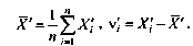
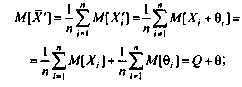
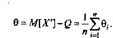
Поскольку неисправленные результаты наблюдений включают в себя систематические погрешности, сумму которых для каждого /-го наблюдения будем обозначать через 8., то их математическое ожидание не совпадает с истинным значением измеряемой величины и отличается от него на некоторую величину 0, называемую систематической погрешностью неисправленного среднего арифметического. Действительно,

Если систематические погрешности постоянны, т.е. 0_/ = 0, /=1,2, …, п, то неисправленные отклонения могут быть непосредственно использованы для оценки рассеивания ряда наблюдений. В противном случае необходимо предварительно исправить отдельные результаты измерений, введя в них так называемые поправки, равные систематическим погрешностям по величине и обратные им по знаку:

q = -Oi.

Таким образом, для нахождения исправленного среднего арифметического и оценки его рассеивания относительно истинного значения измеряемой величины необходимо обнаружить систематические погрешности и исключить их путем введения поправок или соответствующей каждому конкретному случаю организации самого измерения. Остановимся подробнее на некоторых способах обнаружения систематических погрешностей.

Постоянные систематические погрешности не влияют на значения случайных отклонений результатов наблюдений от средних арифметических, поэтому никакая математическая обработка результатов наблюдений не может привести к их обнаружению. Анализ таких погрешностей возможен только на основании некоторых априорных знаний об этих погрешностях, получаемых, например, при поверке средств измерений. Измеряемая величина при поверке обычно воспроизводится образцовой мерой, действительное значение которой известно. Поэтому разность между средним арифметическим результатов наблюдения и значением меры с точностью, определяемой погрешностью аттестации меры и случайными погрешностями измерения, равна искомой систематической погрешности.

Одним из наиболее действенных способов обнаружения систематических погрешностей в ряде результатов наблюдений является построение графика последовательности неисправленных значений случайных отклонений результатов наблюдений от средних арифметических.

Рассматриваемый способ обнаружения постоянных систематических погрешностей можно сформулировать следующим образом: если неисправленные отклонения результатов наблюдений резко изменяются при изменении условий наблюдений, то данные результаты содержат постоянную систематическую погрешность, зависящую от условий наблюдений.

Систематические погрешности являются детерминированными величинами, поэтому в принципе всегда могут быть вычислены и исключены из результатов измерений. После исключения систематических погрешностей получаем исправленные средние арифметические и исправленные отклонения результатов наблюдении, которые позволяют оценить степень рассеивания результатов.

Для исправления результатов наблюдений их складывают с поправками, равными систематическим погрешностям по величине и обратными им по знаку. Поправку определяют экспериментально при поверке приборов или в результате специальных исследований, обыкновенно с некоторой ограниченной точностью.

Поправки могут задаваться также в виде формул, по которым они вычисляются для каждого конкретного случая. Например, при измерениях и поверках с помощью образцовых манометров следует вводить поправки к их показаниям на местное значение ускорения свободного падения

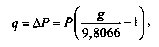
где Р — измеряемое давление.

Введением поправки устраняется влияние только одной вполне определенной систематической погрешности, поэтому в результаты измерения зачастую приходится вводить очень большое число поправок. При этом вследствие ограниченной точности определения поправок накапливаются случайные погрешности и дисперсия результата измерения увеличивается.

Систематическая погрешность, остающаяся после введения поправок на ее наиболее существенные составляющие включает в себя ряд элементарных составляющих, называемых неисключенными остатками систематической погрешности. К их числу относятся погрешности:

• определения поправок;

• зависящие от точности измерения влияющих величин, входящих в формулы для определения поправок;

• связанные с колебаниями влияющих величин (температуры окружающей среды, напряжения питания и т.д.).

Перечисленные погрешности малы, и поправки на них не вводятся.

Свойства физического объекта (явления, процесса) определяются набором
количественных характеристик — физических величин.
Как правило, результат измерения представляет
собой число, задающее отношение измеряемой величины к некоторому эталону.
Сравнение с эталоном может быть как
прямым (проводится непосредственно
экспериментатором), так и косвенным (проводится с помощью некоторого
прибора, которому экспериментатор доверяет).
Полученные таким образом величины имеют размерность, определяемую выбором эталона.

Замечание. Результатом измерения может также служить количество отсчётов некоторого
события, логическое утверждение (да/нет) или даже качественная оценка
(сильно/слабо/умеренно). Мы ограничимся наиболее типичным для физики случаем,
когда результат измерения может быть представлен в виде числа или набора чисел.

Взаимосвязь между различными физическими величинами может быть описана
физическими законами, представляющими собой идеализированную
модель действительности. Конечной целью любого физического
эксперимента (в том числе и учебного) является проверка адекватности или
уточнение параметров таких моделей.

1.1 Результат измерения

Рассмотрим простейший пример: измерение длины стержня
с помощью линейки. Линейка проградуирована производителем с помощью
некоторого эталона длины — таким образом, сравнивая длину
стержня с ценой деления линейки, мы выполняем косвенное сравнение с
общепринятым стандартным эталоном.

Допустим, мы приложили линейку к стержню и увидели на шкале некоторый результат
x=xизм. Можно ли утверждать, что xизм — это длина
стержня?

Во-первых, значение x не может быть задано точно, хотя бы
потому, что оно обязательно округлено до некоторой значащей
цифры: если линейка «обычная», то у неё
есть цена деления; а если линейка, к примеру, «лазерная»
— у неё высвечивается конечное число значащих цифр
на дисплее.

Во-вторых, мы никак не можем быть уверенны, что длина стержня на
самом деле такова хотя бы с точностью до ошибки округления. Действительно,
мы могли приложить линейку не вполне ровно; сама линейка могла быть
изготовлена не вполне точно; стержень может быть не идеально цилиндрическим
и т.п.

И, наконец, если пытаться хотя бы гипотетически переходить к бесконечной
точности измерения, теряет смысл само понятие «длины стержня». Ведь
на масштабах атомов у стержня нет чётких границ, а значит говорить о его
геометрических размерах в таком случае крайне затруднительно!

Итак, из нашего примера видно, что никакое физическое измерение не может быть
произведено абсолютно точно, то есть
у любого измерения есть погрешность.

Замечание. Также используют эквивалентный термин ошибка измерения
(от англ. error). Подчеркнём, что смысл этого термина отличается от
общеупотребительного бытового: если физик говорит «в измерении есть ошибка»,
— это не означает, что оно неправильно и его надо переделать.
Имеется ввиду лишь, что это измерение неточно, то есть имеет
погрешность.

Количественно погрешность можно было бы определить как разность между
измеренным и «истинным» значением длины стержня:
δ⁢x=xизм-xист. Однако на практике такое определение
использовать нельзя: во-первых, из-за неизбежного наличия
погрешностей «истинное» значение измерить невозможно, и во-вторых, само
«истинное» значение может отличаться в разных измерениях (например, стержень
неровный или изогнутый, его торцы дрожат из-за тепловых флуктуаций и т.д.).
Поэтому говорят обычно об оценке погрешности.

Об измеренной величине также часто говорят как об оценке, подчеркивая,
что эта величина не точна и зависит не только от физических свойств
исследуемого объекта, но и от процедуры измерения.

Замечание.
Термин оценка имеет и более формальное значение. Оценкой называют результат процедуры получения значения параметра или параметров физической модели, а также иногда саму процедуру. Теория оценок является подразделом математической статистики. Некоторые ее положения изложены в главе 3, но для более серьезного понимания следует обратиться к [5].

Для оценки значения физической величины корректно использовать
не просто некоторое фиксированное число xизм, а интервал (или
диапазон) значений, в пределах которого может лежать её
«истинное» значение. В простейшем случае этот интервал
может быть записан как

где δ⁢x — абсолютная величина погрешности.
Эта запись означает, что исследуемая величина лежит в интервале
x∈(xизм-δ⁢x;xизм+δ⁢x)
с некоторой достаточно большой долей вероятности (более подробно о
вероятностном содержании интервалов см. п. 2.2).
Для наглядной оценки точности измерения удобно также использовать
относительную величину погрешности:

Она показывает, насколько погрешность мала по сравнению с
самой измеряемой величиной (её также можно выразить в процентах:
ε=δ⁢xx⋅100%).

Пример. Штангенциркуль —
прибор для измерения длин с ценой деления 0,1⁢мм. Пусть
диаметр некоторой проволоки равен 0,37 мм. Считая, что абсолютная
ошибка составляет половину цены деления прибора, результат измерения
можно будет записать как d=0,40±0,05⁢мм (или
d=(40±5)⋅10-5⁢м).
Относительная погрешность составляет ε≈13%, то
есть точность измерения весьма посредственная — поскольку
размер объекта близок к пределу точности прибора.

О необходимости оценки погрешностей.

Измерим длины двух стержней x1 и x2 и сравним результаты.
Можно ли сказать, что стержни одинаковы или различны?

Казалось бы,
достаточно проверить, справедливо ли x1=x2. Но никакие
два результата измерения не равны друг другу с абсолютной точностью! Таким
образом, без указания погрешности измерения ответ на этот вопрос дать
невозможно.

С другой стороны, если погрешность δ⁢x известна, то можно
утверждать, что если измеренные длины одинаковы
в пределах погрешности опыта, если |x2-x1|<δ⁢x
(и различны в противоположном случае).

Итак, без знания погрешностей невозможно сравнить между собой никакие
два измерения, и, следовательно, невозможно сделать никаких
значимых выводов по результатам эксперимента: ни о наличии зависимостей
между величинами, ни о практической применимости какой-либо теории,
и т. п. В связи с этим задача правильной оценки погрешностей является крайне
важной, поскольку существенное занижение или завышение значения погрешности
(по сравнению с реальной точностью измерений) ведёт к неправильным выводам.

В физическом эксперименте (в том числе лабораторном практикуме) оценка
погрешностей должна проводиться всегда
(даже когда составители задания забыли упомянуть об этом).

1.2 Многократные измерения

Проведём серию из n одинаковых (однотипных) измерений одной
и той же физической величины (например, многократно приложим линейку к стержню) и получим
ряд значений

Что можно сказать о данном наборе чисел и о длине стержня?
И можно ли увеличивая число измерений улучшить конечный результат?

Если цена деления самой линейки достаточно мала, то как нетрудно убедиться
на практике, величины {xi} почти наверняка окажутся
различными. Причиной тому могут быть
самые разные обстоятельства, например: у нас недостаточно остроты
зрения и точности рук, чтобы каждый раз прикладывать линейку одинаково;
стенки стержня могут быть слегка неровными; у стержня может и не быть
определённой длины, например, если в нём возбуждены звуковые волны,
из-за чего его торцы колеблются, и т. д.

В такой ситуации результат измерения интерпретируется как
случайная величина, описываемая некоторым вероятностным законом
(распределением).
Подробнее о случайных величинах и методах работы с ними см. гл. 2.

По набору результатов 𝐱 можно вычислить их среднее арифметическое:

⟨x⟩=x1+x2+…+xnn≡1n⁢∑i=1nxi.

(1.1)

Это значение, вычисленное по результатам конечного числа n измерений,
принято называть выборочным средним. Здесь и далее для обозначения
выборочных средних будем использовать угловые скобки.

Кроме среднего представляет интерес и то, насколько сильно варьируются
результаты от опыта к опыту. Определим отклонение каждого измерения от среднего как

Разброс данных относительно среднего принято характеризовать
среднеквадратичным отклонением:

s=Δ⁢x12+Δ⁢x22+…+Δ⁢xn2n=1n⁢∑i=1nΔ⁢xi2

(1.2)

или кратко

Значение среднего квадрата отклонения s2 называют
выборочной дисперсией.

Будем увеличивать число измерений n (n→∞). Если объект измерения и методика
достаточно стабильны, то отклонения от среднего Δ⁢xi будут, во-первых,
относительно малы, а во-вторых, положительные и отрицательные отклонения будут
встречаться примерно одинаково часто. Тогда при вычислении (1.1)
почти все отклонения Δ⁢xi скомпенсируются и можно ожидать,
что выборочное среднее при n≫1 будет стремиться к некоторому пределу:

Тогда предельное значение x¯ можно отождествить с «истинным» средним
для исследуемой величины.

Предельную величину среднеквадратичного отклонения при n→∞
обозначим как

Замечание. В общем случае указанные пределы могут и не существовать. Например, если измеряемый параметр
меняется во времени или в результате самого измерения, либо испытывает слишком большие
случайные скачки и т. п. Такие ситуации требуют особого рассмотрения и мы на них не
останавливаемся.

Замечание. Если n мало (n<10), для оценки среднеквадратичного отклонения
математическая статистика рекомендует вместо формулы (1.3) использовать
исправленную формулу (подробнее см. п. 5.2):

sn-12=1n-1⁢∑i=1nΔ⁢xi2,

(1.4)

где произведена замена n→n-1. Величину sn-1
часто называют стандартным отклонением.

Итак, можно по крайней мере надеяться на то, что результаты небольшого числа
измерений имеют не слишком большой разброс, так что величина ⟨x⟩
может быть использована как приближенное значение (оценка) истинного значения
⟨x⟩≈x¯,
а увеличение числа измерений позволит уточнить результат.

Многие случайные величины подчиняются так называемому нормальному закону
распределения (подробнее см. Главу 2). Для таких величин
могут быть строго доказаны следующие свойства:

•

при многократном повторении эксперимента бо́льшая часть измерений
(∼68%) попадает в интервал x¯-σ<x<x¯+σ
(см. п. 2.2).
•

выборочное среднее значение ⟨x⟩ оказывается с большей
вероятностью ближе к истинному значению x¯, чем каждое из измерений
{xi} в отдельности. При этом ошибка вычисления среднего
убывает пропорционально корню из числа опытов n
(см. п. 2.4).

Упражнение. Показать, что

s2=⟨x2⟩-⟨x⟩2.

(1.5)

то есть дисперсия равна разности среднего значения квадрата
⟨x2⟩=1n⁢∑i=1nxi2
и квадрата среднего ⟨x⟩2=(1n⁢∑i=1nxi)2.

1.3 Классификация погрешностей

Чтобы лучше разобраться в том, нужно ли многократно повторять измерения,
и в каком случае это позволит улучшить результаты опыта,
проанализируем источники и виды погрешностей.

В первую очередь, многократные измерения позволяют проверить
воспроизводимость результатов: повторные измерения в одинаковых
условиях, должны давать близкие результаты. В противном случае
исследование будет существенно затруднено, если вообще возможно.
Таким образом, многократные измерения необходимы для того,
чтобы убедиться как в надёжности методики, так и в существовании измеряемой
величины как таковой.

При любых измерениях возможны грубые ошибки — промахи
(англ. miss). Это «ошибки» в стандартном
понимании этого слова — возникающие по вине экспериментатора
или в силу других непредвиденных обстоятельств (например, из-за сбоя
аппаратуры). Промахов, конечно, нужно избегать, а результаты таких
измерений должны быть по возможности исключены из рассмотрения.

Как понять, является ли «аномальный» результат промахом? Вопрос этот весьма
непрост. В литературе существуют статистические
критерии отбора промахов, которыми мы, однако, настоятельно не рекомендуем
пользоваться (по крайней мере, без серьезного понимания последствий
такого отбора). Отбрасывание аномальных данных может, во-первых, привести
к тенденциозному искажению результата исследований, а во-вторых, так
можно упустить открытие неизвестного эффекта. Поэтому при научных
исследованиях необходимо максимально тщательно проанализировать причину
каждого промаха, в частности, многократно повторив эксперимент. Лишь
только если факт и причина промаха установлены вполне достоверно,
соответствующий результат можно отбросить.

Замечание. Часто причины аномальных отклонений невозможно установить на этапе
обработки данных, поскольку часть информации о проведении измерений к этому моменту
утеряна. Единственным способ борьбы с этим — это максимально подробное описание всего
процесса измерений в лабораторном журнале. Подробнее об этом
см. п. 4.1.1.

При многократном повторении измерении одной и той же физической величины
погрешности могут иметь систематический либо случайный
характер. Назовём погрешность систематической, если она повторяется
от опыта к опыту, сохраняя свой знак и величину, либо закономерно
меняется в процессе измерений. Случайные (или статистические)
погрешности меняются хаотично при повторении измерений как по величине,
так и по знаку, и в изменениях не прослеживается какой-либо закономерности.

Кроме того, удобно разделять погрешности по их происхождению. Можно
выделить

•

инструментальные (или приборные) погрешности,
связанные с несовершенством конструкции (неточности, допущенные при
изготовлении или вследствие старения), ошибками калибровки или ненормативными
условиями эксплуатации измерительных приборов;
•

методические погрешности, связанные с несовершенством
теоретической модели явления (использование приближенных формул и
моделей явления) или с несовершенством методики измерения (например,
влиянием взаимодействия прибора и объекта измерения на результат измерения);
•

естественные погрешности, связанные со случайным
характером
измеряемой физической величины — они являются не столько
«ошибками» измерения, сколько характеризуют
природу изучаемого объекта или явления.

Замечание. Разделение погрешностей на систематические и случайные
не является однозначным и зависит от постановки опыта. Например, производя
измерения не одним, а несколькими однотипными приборами, мы переводим
систематическую приборную ошибку, связанную с неточностью шкалы и
калибровки, в случайную. Разделение по происхождению также условно,
поскольку любой прибор подвержен воздействию «естественных»
случайных и систематических ошибок (шумы и наводки, тряска, атмосферные
условия и т. п.), а в основе работы прибора всегда лежит некоторое
физическое явление, описываемое не вполне совершенной теорией.

1.3.1 Случайные погрешности

Случайный характер присущ большому количеству различных физических
явлений, и в той или иной степени проявляется в работе всех без исключения
приборов. Случайные погрешности обнаруживаются просто при многократном
повторении опыта — в виде хаотичных изменений (флуктуаций)
значений {xi}.

Если случайные отклонения от среднего в большую или меньшую стороны
примерно равновероятны, можно рассчитывать, что при вычислении среднего
арифметического (1.1) эти отклонения скомпенсируются,
и погрешность результирующего значения ⟨x⟩ будем меньше,
чем погрешность отдельного измерения.

Случайные погрешности бывают связаны, например,

•

с особенностями используемых приборов: техническими
недостатками
(люфт в механических приспособлениях, сухое трение в креплении стрелки
прибора), с естественными (тепловой и дробовой шумы в электрических
цепях, тепловые флуктуации и колебания измерительных устройств из-за
хаотического движения молекул, космическое излучение) или техногенными
факторами (тряска, электромагнитные помехи и наводки);
•

с особенностями и несовершенством методики измерения (ошибка
при отсчёте по шкале, ошибка времени реакции при измерениях с секундомером);
•

с несовершенством объекта измерений (неровная поверхность,
неоднородность состава);
•

со случайным характером исследуемого явления (радиоактивный
распад, броуновское движение).

Остановимся несколько подробнее на двух последних случаях. Они отличаются
тем, что случайный разброс данных в них порождён непосредственно объектом
измерения. Если при этом приборные погрешности малы, то «ошибка»
эксперимента возникает лишь в тот момент, когда мы по своей
воле совершаем замену ряда измеренных значений на некоторое среднее
{xi}→⟨x⟩. Разброс данных при этом
характеризует не точность измерения, а сам исследуемый объект или
явление. Однако с математической точки зрения приборные и
«естественные»
погрешности неразличимы — глядя на одни только
экспериментальные данные невозможно выяснить, что именно явилось причиной
их флуктуаций: сам объект исследования или иные, внешние причины.
Таким образом, для исследования естественных случайных процессов необходимо
сперва отдельно исследовать и оценить случайные инструментальные погрешности
и убедиться, что они достаточно малы.

1.3.2 Систематические погрешности

Систематические погрешности, в отличие от случайных, невозможно обнаружить,
исключить или уменьшить просто многократным повторением измерений.
Они могут быть обусловлены, во-первых, неправильной работой приборов
(инструментальная погрешность), например, сдвигом нуля отсчёта
по шкале, деформацией шкалы, неправильной калибровкой, искажениями
из-за не нормативных условий эксплуатации, искажениями из-за износа
или деформации деталей прибора, изменением параметров прибора во времени
из-за нагрева и т.п. Во-вторых, их причиной может быть ошибка в интерпретации
результатов (методическая погрешность), например, из-за использования
слишком идеализированной физической модели явления, которая не учитывает
некоторые значимые факторы (так, при взвешивании тел малой плотности
в атмосфере необходимо учитывать силу Архимеда; при измерениях в электрических
цепях может быть необходим учет неидеальности амперметров и вольтметров
и т. д.).

Систематические погрешности условно можно разделить на следующие категории.

1.

Известные погрешности, которые могут быть достаточно точно вычислены
или измерены. При необходимости они могут быть учтены непосредственно:
внесением поправок в расчётные формулы или в результаты измерений.
Если они малы, их можно отбросить, чтобы упростить вычисления.
2.

Погрешности известной природы, конкретная величина которых неизвестна,
но максимальное значение вносимой ошибки может быть оценено теоретически
или экспериментально. Такие погрешности неизбежно присутствуют в любом
опыте, и задача экспериментатора — свести их к минимуму,
совершенствуя методики измерения и выбирая более совершенные приборы.

Чтобы оценить величину систематических погрешностей опыта, необходимо
учесть паспортную точность приборов (производитель, как правило, гарантирует,
что погрешность прибора не превосходит некоторой величины), проанализировать
особенности методики измерения, и по возможности, провести контрольные
опыты.
3.

Погрешности известной природы, оценка величины которых по каким-либо
причинам затруднена (например, сопротивление контактов при подключении
электронных приборов). Такие погрешности должны быть обязательно исключены
посредством модификации методики измерения или замены приборов.
4.

Наконец, нельзя забывать о возможности существования ошибок, о
которых мы не подозреваем, но которые могут существенно искажать результаты
измерений. Такие погрешности самые опасные, а исключить их можно только
многократной независимой проверкой измерений, разными методами
и в разных условиях.

В учебном практикуме учёт систематических погрешностей ограничивается,
как правило, паспортными погрешностями приборов и теоретическими поправками
к упрощенной модели исследуемого явления.

Точный учет систематической ошибки возможен только при учете специфики конкретного эксперимента. Особенное внимание надо обратить на зависимость (корреляцию) систематических смещений при повторных измерениях. Одна и та же погрешность в разных случаях может быть интерпретирована и как случайная, и как систематическая.

Пример.
Калибровка электромагнита производится при помощи внесения в него датчика Холла или другого измерителя магнитного потока. При последовательных измерениях с разными токами (и соотственно полями в зазоре) калибровку можно учитыать двумя различными способами:

•

Измерить значение поля для разных токов, построить линейную калибровочную кривую и потом использовать значения, восстановленные по этой кривой для вычисления поля по току, используемому в измерениях.

•

Для каждого измерения проводить допольнительное измерения поля и вообще не испльзовать значения тока.

В первом случае погрешность полученного значения будет меньше, поскльку при проведении прямой, отдельные отклонения усреднятся. При этом погрешность измерения поля будет носить систематический харрактер и при обработке данных ее надо будет учитывать в последний момент. Во втором случае погрешность будет носить статистический (случайный) харрактер и ее надо будет добавить к погрешности каждой измеряемой точки. При этом сама погрешность будет больше. Выбор той или иной методики зависит от конретной ситуации. При большом количестве измерений, второй способ более надежный, поскольку статистическая ошибка при усреднении уменьшается пропорционально корню из количества измерений. Кроме того, такой способ повзоляет избежать методической ошибки, связанной с тем, что зависимость поля от тока не является линейной.

Пример.
Рассмотрим измерение напряжения по стрелочному вольтметру. В показаниях прибора будет присутствовать три типа погрешности:

1.

Статистическая погрешность, связанная с дрожанием стрелки и ошибкой визуального наблюдения, примерно равная половине цены деления.

2.

Систематическая погрешность, связанная с неправильной установкой нуля.

3.

Систематическая погрешность, связанная с неправильным коэффициентом пропорциональности между напряжением и отклонением стрелки. Как правило приборы сконструированы таким образом, чтобы максимальное значение этой погрешности было так же равно половине цены деления (хотя это и не гарантируется).

Неотъемлемой частью любого измерения является погрешность измерений. С развитием приборостроения и методик измерений человечество стремиться снизить влияние данного явления на конечный результат измерений. Предлагаю более детально разобраться в вопросе, что же это такое погрешность измерений.

Погрешность измерения – это отклонение результата измерения от истинного значения измеряемой величины. Погрешность измерений представляет собой сумму погрешностей, каждая из которых имеет свою причину.

По форме числового выражения погрешности измерений подразделяются на абсолютные и относительные

Абсолютная погрешность – это погрешность, выраженная в единицах измеряемой величины. Она определяется выражением.

(1.2), где X — результат измерения; Х₀ — истинное значение этой величины.

Поскольку истинное значение измеряемой величины остается неизвестным, на практике пользуются лишь приближенной оценкой абсолютной погрешности измерения, определяемой выражением

(1.3), где Х_д — действительное значение этой измеряемой величины, которое с погрешностью ее определения принимают за истинное значение.

Относительная погрешность – это отношение абсолютной погрешности измерения к действительному значению измеряемой величины:

(1.4)

По закономерности появления погрешности измерения подразделяются на систематические, прогрессирующие, и случайные.

Систематическая погрешность – это погрешность измерения, остающаяся постоянной или закономерно изменяющейся при повторных измерениях одной и той же величины.

Прогрессирующая погрешность – это непредсказуемая погрешность, медленно меняющаяся во времени.

Систематические и прогрессирующие погрешности средств измерений вызываются:

первые — погрешностью градуировки шкалы или ее небольшим сдвигом;
вторые — старением элементов средства измерения.

Систематическая погрешность остается постоянной или закономерно изменяющейся при многократных измерениях одной и той же величины. Особенность систематической погрешности состоит в том, что она может быть полностью устранена введением поправок. Особенностью прогрессирующих погрешностей является то, что они могут быть скорректированы только в данный момент времени. Они требуют непрерывной коррекции.

Случайная погрешность – это погрешность измерения изменяется случайным образом. При повторных измерениях одной и той же величины. Случайные погрешности можно обнаружить только при многократных измерениях. В отличии от систематических погрешностей случайные нельзя устранить из результатов измерений.

По происхождению различают инструментальные и методические погрешности средств измерений.

Инструментальные погрешности — это погрешности, вызываемые особенностями свойств средств измерений. Они возникают вследствие недостаточно высокого качества элементов средств измерений. К данным погрешностям можно отнести изготовление и сборку элементов средств измерений; погрешности из-за трения в механизме прибора, недостаточной жесткости его элементов и деталей и др. Подчеркнем, что инструментальная погрешность индивидуальна для каждого средства измерений.

Методическая погрешность — это погрешность средства измерения, возникающая из-за несовершенства метода измерения, неточности соотношения, используемого для оценки измеряемой величины.

Погрешности средств измерений.

Абсолютная погрешность меры – это разность между номинальным ее значением и истинным (действительным) значением воспроизводимой ею величины:

(1.5), где X_н – номинальное значение меры; Х_д – действительное значение меры

Абсолютная погрешность измерительного прибора – это разность между показанием прибора и истинным (действительным) значением измеряемой величины:

(1.6), где X_п – показания прибора; Х_д – действительное значение измеряемой величины.

Относительная погрешность меры или измерительного прибора – это отношение абсолютной погрешности меры или измерительного прибора к истинному

(действительному) значению воспроизводимой или измеряемой величины. Относительная погрешность меры или измерительного прибора может быть выражена в ( % ).

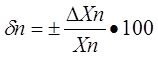(1.7)

Приведенная погрешность измерительного прибора – отношение погрешности измерительного прибора к нормирующему значению. Нормирующие значение XN – это условно принятое значение, равное или верхнему пределу измерений, или диапазону измерений, или длине шкалы. Приведенная погрешность обычно выражается в ( % ).

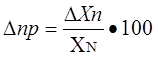(1.8)

Предел допускаемой погрешности средств измерений – наибольшая без учета знака погрешность средства измерений, при которой оно может быть признано и допущено к применению. Данное определение применяют к основной и дополнительной погрешности, а также к вариации показаний. Поскольку свойства средств измерений зависят от внешних условий, их погрешности также зависят от этих условий, поэтому погрешности средств измерений принято делить на основные и дополнительные.

Основная – это погрешность средства измерений, используемого в нормальных условиях, которые обычно определены в нормативно-технических документах на данное средство измерений.

Дополнительная – это изменение погрешности средства измерений вследствии отклонения влияющих величин от нормальных значений.

Погрешности средств измерений подразделяются также на статические и динамические.

Статическая – это погрешность средства измерений, используемого для измерения постоянной величины. Если измеряемая величина является функцией времени, то вследствие инерционности средств измерений возникает составляющая общей погрешности, называется динамической погрешностью средств измерений.

Также существуют систематические и случайные погрешности средств измерений они аналогичны с такими же погрешностями измерений.

Факторы влияющие на погрешность измерений.

Погрешности возникают по разным причинам: это могут быть ошибки экспериментатора или ошибки из-за применения прибора не по назначению и т.д. Существует ряд понятий которые определяют факторы влияющие на погрешность измерений

Вариация показаний прибора – это наибольшая разность показаний полученных при прямом и обратном ходе при одном и том же действительном значении измеряемой величины и неизменных внешних условиях.

Класс точности прибора – это обобщенная характеристика средств измерений (прибора), определяемая пределами допускаемых основной и дополнительных погрешностей, а также другими свойствами средств измерений, влияющих на точность, значение которой устанавливаются на отдельные виды средств измерений.

Классы точности прибора устанавливают при выпуске, градуируя его по образцовому прибору в нормальных условиях.

Прецизионность — показывает, как точно или отчетливо можно произвести отсчет. Она определяется, тем насколько близки друг к другу результаты двух идентичных измерений.

Разрешение прибора — это наименьшее изменение измеряемого значения, на которое прибор будет реагировать.

Диапазон прибора — определяется минимальным и максимальным значением входного сигнала, для которого он предназначен.

Полоса пропускания прибора — это разность между минимальной и максимальной частотой, для которых он предназначен.

Чувствительность прибора — определяется, как отношение выходного сигнала или показания прибора к входному сигналу или измеряемой величине.

Шумы — любой сигнал не несущий полезной информации.

Источник

(6)

(7)

В
случае рассматриваемой нами работы N
24 =0.26
см,
а
равна либо 0.05 см,
либо 0.5 см.
В этом случае

Как
видно, в первом случае можно пренебречь
,
а во втором .

Соседние файлы в папке физика

#
#
29.03.201687.04 Кб6mekh1.doc
#
#
#
#

В зависимости от причин возникновения рассматриваются четыре вида систематических погрешностей.

Среди переменных систематических погрешностей принято выделять прогрессивные и периодические.

q = -Oi.

где Р — измеряемое давление.

• определения поправок;

• зависящие от точности измерения влияющих величин, входящих в формулы для определения поправок;

• связанные с колебаниями влияющих величин (температуры окружающей среды, напряжения питания и т.д.).

Перечисленные погрешности малы, и поправки на них не вводятся.

Experimental techniques

Yanqiu Huang, … Zhixiang Cao, in Industrial Ventilation Design Guidebook (Second Edition), 2021

4.3.3.2 Measurement errors

The measurement errors are divided into two categories: systematic errors and random errors (OIML, 1978).

Systematic error is an error which, in the course of a number of measurements carried out under the same conditions of a given value and quantity, either remains constant in absolute value and sign, or varies according to definite law with changing conditions.

Random error varies in an unpredictable manner in absolute value and in sign when a large number of measurements of the same value of a quantity are made under essentially identical conditions.

The origins of the above two errors are different in cause and nature. A simple example is when the mass of a weight is less than its nominal value, a systematic error occurs, which is constant in absolute value and sign. This is a pure systematic error. A ventilation-related example is when the instrument factor of a Pitot-static tube, which defines the relationship between the measured pressure difference and the velocity, is incorrect, a systematic error occurs. On the other hand, if a Pitot-static tube is positioned manually in a duct in such a way that the tube tip is randomly on either side of the intended measurement point, a random error occurs. This way, different phenomena create different types of error. The (total) error of measurement usually is a combination of the above two types.

The question may be asked, that is, what is the reason for dividing the errors into two categories? The answer is the totally different way of dealing with these different types. Systematic error can be eliminated to a sufficient degree, whereas random error cannot. The following section shows how to deal with these errors.

Read full chapter

URL:

https://www.sciencedirect.com/science/article/pii/B9780128166734000043

EXPERIMENTAL TECHNIQUES

KAI SIREN, … PETER V. NIELSEN, in Industrial Ventilation Design Guidebook, 2001

12.3.3.11 Systematic Errors

Systematic error, as stated above, can be eliminated—not totally, but usually to a sufficient degree. This elimination process is called “calibration.” Calibration is simply a procedure where the result of measurement recorded by an instrument is compared with the measurement result of a standard. A standard is a measuring device intended to define, to represent physically, to conserve, or to reproduce the unit of measurement in order to transmit it to other measuring instruments by comparison.¹ There are several categories of standards, but, simplifying a little, a standard is an instrument with a very high accuracy and can for that reason be used as a reference for ordinary measuring instruments. The calibration itself is usually carried out by measuring the quantity over the whole range required and by defining either one correction factor for the whole range, for a constant systematic error, or a correction curve or equation for the whole range. Applying this correction to the measurement result eliminates, more or less, the systematic error and gives the corrected result of measurement.

A primary standard has the highest metrological quality in a given field. Hence, the primary standard is the most accurate way to measure or to reproduce the value of a quantity. Primary standards are usually complicated instruments, which are essentially laboratory instruments and unsuited for site measurement. They require skilled handling and can be expensive. For these reasons it is not practical to calibrate all ordinary meters against a primary standard. To utilize the solid metrological basis of the primary standard, a chain of secondary standards, reference standards, and working standards combine the primary standard and the ordinary instruments. The lower level standard in the chain is calibrated using the next higher level standard. This is called “traceability.” In all calibrations traceability along the chain should exist, up to the instrument with the highest reliability, the primary standard.

The question is often asked, How often should calibration be carried out? Is it sufficient to do it once, or should it be repeated? The answer to this question depends on the instrument type. A very simple instrument that is robust and stable may require calibrating only once during its lifetime. Some fundamental meters do not need calibration at all. A Pitot-static tube or a liquid U-tube manometer are examples of such simple instruments. On the other hand, complicated instruments with many components or sensitive components may need calibration at short intervals. Also fouling and wearing are reasons not only for maintenance but also calibration. Thus the proper calibration interval depends on the instrument itself and its use. The manufacturers recommendations as well as past experience are often the only guidelines.

Read full chapter

URL:

https://www.sciencedirect.com/science/article/pii/B9780122896767500151

Intelligent control and protection in the Russian electric power system

Nikolai Voropai, … Daniil Panasetsky, in Application of Smart Grid Technologies, 2018

3.3.1.2 Systematic errors in PMU measurements

The systematic errors caused by the errors of the instrument transformers that exceed the class of their accuracy are constantly present in the measurements and can be identified by considering some successive snapshots of measurements. The TE linearized at the point of a true measurement, taking into account random and systematic errors, can be written as:

(25)wky¯=∑l∈ωk∂w∂ylξyl+cyl=∑aklξyl+∑aklcyl

where ∑ a_klξ_{y_l}—mathematical expectation of random errors of the TE, equal to zero; ∑ a_klc_{y_l}—mathematical expectation of systematic error of the TE, ω_k—a set of measurements contained in the kth TE.

The author of Ref. [28] suggests an algorithm for the identification of a systematic component of the measurement error on the basis of the current discrepancy of the TE. The algorithm rests on the fact that systematic errors of measurements do not change through a long time interval. In this case, condition (17) will not be met during such an interval of time. Based on the snapshots that arrive at time instants 0, 1, 2, …, t − 1, t…, the sliding average method is used to calculate the mathematical expectation of the TE discrepancy:

(26)Δwkt=1−αΔwkt−1+αwkt

where 0 ≤ α ≤ 1.

Fig. 5 shows the curve of the TE discrepancy (a thin dotted line) calculated by (26) for 100 snapshots of measurements that do not have systematic errors.

Fig. 5

Fig. 5. Detection of a systematic error in the PMU measurements and identification of mathematical expectation of the test equation.

It virtually does not exceed the threshold d_k = 0.014 (a light horizontal line). Above the threshold, there is a curve of the TE discrepancy (a bold dotted line) that contains a measurement with a systematic error and a curve of nonzero mathematical expectation Δ_{w_k}(t) ∈ [0.026; 0.03] (a black-blue thick line). However, the nonzero value of the calculated mathematical expectation of the TE discrepancy can only testify to the presence of a systematic error in the PMU measurements contained in this TE, but cannot be used to locate it.

Read full chapter

URL:

https://www.sciencedirect.com/science/article/pii/B9780128031285000039

Measurements

Sankara Papavinasam, in Corrosion Control in the Oil and Gas Industry, 2014

ii Systematic or determinate error

To define systematic error, one needs to understand ‘accuracy’. Accuracy is a measure of the closeness of the data to its true or accepted value. Figure 12.3 illustrates accuracy schematically.⁴ Determining the accuracy of a measurement is difficult because the true value may never be known, so for this reason an accepted value is commonly used. Systematic error moves the mean or average value of a measurement from the true or accepted value.

FIGURE 12.3. Difference between Accuracy and Precision in a Measurement.⁴

Reproduced with permission from Brooks/Cole, A Division of Cengage Learning.

Systematic error may be expressed as absolute error or relative error:

•: The absolute error (E_A) is a measure of the difference between the measured value (x_i) and true or accepted value (x_t) (Eqn. 12.5):

(Eqn. 12.5)EA=xi−xt

Absolute error bears a sign:

•: A negative sign indicates that the measured value is smaller than true value and
•: A positive sign indicates that the measured value is higher than true value

The relative error (E_R) is the ratio of measured value to true value and it is expressed as (Eqn. 12.6):

(Eqn. 12.6)ER=(xi−xtxt).100

Table 12.2 illustrates the absolute and relative errors for six measurements in determining the concentration of 20 ppm of an ionic species in solution.

Table 12.2. Relative and Absolute Errors in Six Measurements of Aqueous Solution Containing 20 ppm of an Ionic Species

Measured Value	Absolute Error	Relative Error (Percentage)	Remarks
19.4	−0.6	−3.0	Experimental value lower than actual value.
19.5	−0.5	−2.5
19.6	−0.4	−2.0
19.8	−0.2	−1.0
20.1	+0.1	+0.5	Experimental value higher than actual value.
20.3	+0.3	+1.5

Systematic error may occur due to instrument, methodology, and personal error.

Instrument error

Instrument error occurs due to variations that can affect the functionality of the instrument. Some common causes include temperature change, voltage fluctuation, variations in resistance, distortion of the container, error from original calibration, and contamination. Most instrument errors can be detected and corrected by frequently calibrating the instrument using a standard reference material. Standard reference materials may occur in different forms including minerals, gas mixtures, hydrocarbon mixtures, polymers, solutions of known concentration of chemicals, weight, and volume. The standard reference materials may be prepared in the laboratory or may be obtained from standard-making organizations (e.g., ASTM standard reference materials), government agencies (e.g., National Institute of Standards and Technology (NIST) provides about 900 reference materials) and commercial suppliers. If standard materials are not available, a blank test may be performed using a solution without the sample. The value from this test may be used to correct the results from the actual sample. However this methodology may not be applicable for correcting instrumental error in all situations.

Methodology error

Methodology error occurs due to the non-ideal physical or chemical behavior of the method. Some common causes include variation of chemical reaction and its rate, incompleteness of the reaction between analyte and the sensing element due to the presence of other interfering substances, non-specificity of the method, side reactions, and decomposition of the reactant due to the measurement process. Methodology error is often difficult to detect and correct, and is therefore the most serious of the three types of systematic error. Therefore a suitable method free from methodology error should be established for routine analysis.

Personal error

Personal error occurs due to carelessness, lack of detailed knowledge of the measurement, limitation (e.g., color blindness of a person performing color-change titration), judgment, and prejudice of person performing the measurement. Some of these can be overcome by automation, proper training, and making sure that the person overcomes any bias to preserve the integrity of the measurement.

Read full chapter

URL:

https://www.sciencedirect.com/science/article/pii/B9780123970220000121

Experimental Design and Sample Size Calculations

Andrew P. King, Robert J. Eckersley, in Statistics for Biomedical Engineers and Scientists, 2019

9.4.2 Blinding

1.: Single-blind. The participant does not know if he/she is a member of the treatment or control group. This normally requires the control group to receive a placebo. Single-blinding can be easy to achieve in some types of experiments, for example, in drug trials the control group could receive sugar pills. However, it can be more difficult for other types of treatment. For example, in surgery there are ethical issues involved in patients having a placebo (or sham) operation.²
2.: Double-blind. Neither the participant nor the researcher who delivers the treatment knows whether the participant is in the treatment or control group.
3.: Triple-blind. Neither the participant, the researcher who delivers the treatment, nor the researcher who measures the response knows whether the participant is in the treatment or control group.

Read full chapter

URL:

https://www.sciencedirect.com/science/article/pii/B9780081029398000189

The pursuit and definition of accuracy

Anthony J. Martyr, David R. Rogers, in Engine Testing (Fifth Edition), 2021

Systematic instrument errors

Typical systematic errors (Fig. 19.2C) include the following:

1.: Zero errors—the instrument does not read zero when the value of the quantity observed is zero.
2.: Scaling errors—the instrument reads systematically high or low.
3.: Nonlinearity—the relation between the true value of the quantity and the indicated value is not exactly in proportion; if the proportion of error is plotted against each measurement over full scale, the graph is nonlinear.
4.: Dimensional errors—for example, the effective length of a dynamometer torque arm may not be precisely correct.

Read full chapter

URL:

https://www.sciencedirect.com/science/article/pii/B978012821226400019X

Power spectrum and filtering

Andreas Skiadopoulos, Nick Stergiou, in Biomechanics and Gait Analysis, 2020

5.10 Practical implementation

As suggested by Winter (2009), to cancel the phase shift of the output signal relative to the input that is introduced by the second-order filter, the once-filtered data has to filtered again, but this time in the reverse direction. However, at every pass the −3dB cutoff frequency is pushed lower, and a correction is needed to match the original single-pass filter. This correction should be applied once the coefficients of the fourth-order low-pass filter are calculated. Nevertheless, it should be also checked whether functions of closed source software use the correction factor. If they have not used it, the output of the analyzed signal will be distorted. The format of the recursive second-order filter is given by Eq. (5.36) (Winter, 2009):

(5.36)yk=α0χk+α1χk−1+α2χk−2+β1yk−1+β2yk−2

where y are the filtered output data, x are past inputs, and k the kth sample.The coefficients α0,α1,α2,β1, and β2 for a second-order Butterworth low-pass filter are computed from Eq. (5.37) (Winter, 2009):

(5.37)ωc=tanπfcfsCK1=2ωcK2=ωc2K3=α1K2α0=K21+K1+K2α1=2α0α2=α0β1=K3−α1β2=1−α1-K3

where, ω_c is the cutoff angular frequency in rad/s, fc is the cutoff frequency in Hz, and fs is the sampling rate in Hz. When the filtered data are filtered again in the reverse direction to cancel phase-shift, the following correction factor to compensate for the introduced error should be used:

(5.38)C=(21n−1)14

where n≥2 is the number of passes. For a single-pass C=1, and no compensation is needed. For a dual pass, (n=2), a compensation is needed, and the correction factor should be applied. Thus, the ωc term from Eq. (5.37) is calculated as follows:

(5.39)ωc=tan(πfcfs)(212−1)14=tan(πfcfs)0.802

A systematic error is introduced to the signal if the correction factor is not applied. Therefore, remember to check any algorithm before using it. Let us check the correctness of the fourth-order low-pass filter that was built previously in R language. Vignette 5.2 contains the code to perform Winter’s (2009) low-pass filter in R programming language. Because the filter needs two past inputs (two data points) to compute a present filtered output (one data point), the time-series data to be filtered (the raw data) should be padded at the beginning and at the end. Additional data are usually collected before and after the period of interest.

Vignette 5.2

The following vignette contains a code in R programming language that performs the fourth-order zero-phase-shift low-pass filter from Eq. (5.37).

1.

The first step is to create a sine (or equally a cosine) wave with known amplitude and known frequency. Vignette 5.3 is used to synthesize periodic digital waves. Let us create a simple periodic sine wave s[n] with the following characteristics:

a.: Amplitude A=1 unit (e.g., 1 m);
b.: Frequency f=2 Hz;
c.: Phase θ=0 rad;
d.: Shift a₀=0 unit (e.g., 0 m).

Vignette 5.3

The following vignette contains a code in R programming language that synthesizes periodic waveforms from sinusoids.

Let us choose an arbitrary fundamental period T₀=2 seconds, which corresponds to a fundamental frequency of f0=1/T0=0.5 Hz. Now, knowing the fundamental frequency, the fourth harmonic that corresponds to a sine wave with frequency of f=2 Hz will be chosen. The periodic sine wave s[n] will be sampled at Fs=40 Hz (T_s=1/40 seconds) (i.e., 20 times the Nyquist frequency, f_N=2 Hz). The sine wave will be recorded for a time interval of t=2 s, which corresponds to N=80 data points. Thus, and because ω₀=2πf₀, we have:

s[n]=sin(2ω0nTs)

which means that the fourth harmonic has frequency f=2

Hz. Fig. 5.14A shows the sine wave created. The first and last 20 data points can be considered as extra points (padded). Additional data at the beginning and end of the signal are needed for the next steps because the filter is does not behave well at the edges. Thus, the signal of interest starts at 0.5

seconds and ends at 1.5

seconds, which corresponds to N=40 data points.

Figure 5.14. (A) Example of a low-pass filter (cutoff frequency=2 Hz) applied to a sine wave sampled at 40 Hz, with amplitude equal to 1 m, and frequency equal to 2 Hz. (B) The signal interpolated by a factor of 2, and filtered with cutoff frequency equal to the frequency of the sine wave (cutoff frequency=2 Hz). (C) Since the amplitude of the filtered signal has been reduced by a ratio of 0.707, the low-pass filter correctly attenuated the signal. The power spectra of the original and reconstructed signal are shown.

2.

An extra, but not mandatory, step is to interpolate the created sine wave in order to increase the temporal resolution of the created signal (Fig. 5.14B). Of course, when a digital periodic signal is created from scratch, like we are doing using the R code in the vignettes, we can easily sample the signal at higher frequencies. However, if we want to use real biomechanical time series data, that have already been collected, a possible way to increase its temporal resolution is by using the Whittaker–Shannon interpolation formula. With the Whittaker–Shannon interpolation a signal is up-sampled with interpolation using the sinc() function (Yaroslavsky, 1997):

(5.40)s(x)=∑n=0N−1αnsin(π(xΔx−n))Nsin(π(xΔx−n)/N)

The Whittaker–Shannon interpolation formula can be used to increase the temporal resolution after removing the “white” noise from the data. Without filtering, the interpolation results in a noise level equal to that of the original signal before sampling (Marks, 1991). However, the interpolation noise can be reduced by both oversampling and filtering the data before interpolation (Marks, 1991). An alternative, and efficient, method is to run the DFT, zero-pad the signal, and then take the IDFT to reconstruct it. Vignette 5.4 can be used to increase the temporal resolution by a factor of 2, which corresponds to a sampling frequency of 80 Hz.

Vignette 5.4

The following vignette contains a code in R programming language that runs the normalized discrete sinc() function, and the Whittaker–Shannon interpolation function.

3.

The third step is to filter the previously created sine wave with the fourth-order zero-phase-shift low-pass filter, setting the cutoff frequency equal to the sine wave frequency f=2 Hz. Vignette 5.2 is used for step 3. To cancel any shift (i.e., a zero-phase-shift filter) n=2 passes must be chosen. The interpolated signal has a sampling rate of 80 Hz.

4.

The fourth step is to investigate the frequency response of the filtered sine wave. The frequency response of the Butterworth filter is given by Eq. (5.41)

(5.41)|AoutAin|=1(1+fsf3dB)2n

where the point at which the amplitude response, Aout, of the input signal, s[n], with frequency, f, and amplitude, A_in, drops off by 3dB and is known as the cutoff frequency, f3dB. When the cutoff frequency is set equal to the frequency of the signal (f_3dB=f), the ratio should be equal to 0.707, since:

(5.42)|AoutAin|=12≈0.707

Fig. 5.14C shows the plots of the filtered and interpolated sine wave. Since the ratio of the maximum value of the filtered sine wave to the original sine wave ratio=0.707, the created fourth-order zero-phase-shift low-pass filter works properly. Without the correction factor the amplitude reduces nearly to half (0.51), indicating that the coefficients of the filter needed correction. Fig. 5.15 also shows an erroneously filtered signal. You can try to create Fig. 5.15 by yourself.

Figure 5.15. Example of a recursive low-pass filter applied to a sine wave with amplitude equal to 1 m and cutoff frequency equal to the frequency of the sine wave. Since the amplitude of the filtered signal has been reduced by a ratio of 0.707, the low-pass filter correctly attenuated the signal. However, the function without the correction factor reduced the amplitude by nearly one-half (0.51), indicating that the coefficients need correction.

The same procedure should be applied to check whether the output of the functions from closed source software used the correction factor or not. For example, using the library(signal) of the R computational software, if x is the vector that contains the raw data, then using butter() the Butterworth coefficients can be generated.

Read full chapter

URL:

https://www.sciencedirect.com/science/article/pii/B9780128133729000051

The Systems Approach to Control and Instrumentation

William B. Ribbens, in Understanding Automotive Electronics (Seventh Edition), 2013

Systematic Errors

One example of a systematic error is known as loading errors, which are due to the energy extracted by an instrument when making a measurement. Whenever the energy extracted from a system under measurement is not negligible, the extracted energy causes a change in the quantity being measured. Wherever possible, an instrument is designed to minimize such loading effects. The idea of loading error can be illustrated by the simple example of an electrical measurement, as illustrated in Figure 1.17. A voltmeter M having resistance R_m measures the voltage across resistance R. The correct voltage (v_c) is given by

Figure 1.17. Illustration of loading error-volt meter.

(71)vc=V(RR+R1)

However, the measured voltage v_m is given by

(72)vm=V(RpRp+R1)

where R_p is the parallel combination of R and R_m:

(73)Rp=RRmR+Rm

Loading is minimized by increasing the meter resistance R_m to the largest possible value. For conditions where R_m approaches infinite resistance, R_p approaches resistance R and v_m approaches the correct voltage. Loading is similarly minimized in measurement of any quantity by minimizing extracted energy. Normally, loading is negligible in modern instrumentation.

Another significant systematic error source is the dynamic response of the instrument. Any instrument has a limited response rate to very rapidly changing input, as illustrated in Figure 1.18. In this illustration, an input quantity to the instrument changes abruptly at some time. The instrument begins responding, but cannot instantaneously change and produce the new value. After a transient period, the indicated value approaches the correct reading (presuming correct instrument calibration). The dynamic response of an instrument to rapidly changing input quantity varies inversely with its bandwidth as explained earlier in this chapter.

Figure 1.18. Illustration of instrument dynamic response error.

In many automotive instrumentation applications, the bandwidth is purposely reduced to avoid rapid fluctuations in readings. For example, the type of sensor used for fuel-quantity measurements actually measures the height of fuel in the tank with a small float. As the car moves, the fuel sloshes in the tank, causing the sensor reading to fluctuate randomly about its mean value. The signal processing associated with this sensor is actually a low-pass filter such as is explained later in this chapter and has an extremely low bandwidth so that only the average reading of the fuel quantity is displayed, thereby eliminating the undesirable fluctuations in fuel quantity measurements that would occur if the bandwidth were not restricted.

The reliability of an instrumentation system refers to its ability to perform its designed function accurately and continuously whenever required, under unfavorable conditions, and for a reasonable amount of time. Reliability must be designed into the system by using adequate design margins and quality components that operate both over the desired temperature range and under the applicable environmental conditions.

Read full chapter

URL:

https://www.sciencedirect.com/science/article/pii/B9780080970974000011

Measurement uncertainty

Alan S. Morris, Reza Langari, in Measurement and Instrumentation (Third Edition), 2021

3.2 Sources of systematic error

The main sources of systematic error in the output of measuring instruments can be summarized as:

(i): effect of environmental disturbances, often called modifying inputs
(ii): disturbance of the measured system by the act of measurement
(iii): changes in characteristics due to wear in instrument components over a period of time
(iv): resistance of connecting leads

These various sources of systematic error, and ways in which the magnitude of the errors can be reduced, are discussed next.

3.2.1 System disturbance due to measurement

Disturbance of the measured system by the act of measurement is a common source of systematic error. If we were to start with a beaker of hot water and wished to measure its temperature with a mercury-in-glass thermometer, then we would take the thermometer, which would initially be at room temperature, and plunge it into the water. In so doing, we would be introducing a relatively cold mass (the thermometer) into the hot water and a heat transfer would take place between the water and the thermometer. This heat transfer would lower the temperature of the water. While the reduction in temperature in this case would be so small as to be undetectable by the limited measurement resolution of such a thermometer, the effect is finite and clearly establishes the principle that, in nearly all measurement situations, the process of measurement disturbs the system and alters the values of the physical quantities being measured.

A particularly important example of this occurs with the orifice plate. This is placed into a fluid-carrying pipe to measure the flow rate, which is a function of the pressure that is measured either side of the orifice plate. This measurement procedure causes a permanent pressure loss in the flowing fluid. The disturbance of the measured system can often be very significant.

Thus, as a general rule, the process of measurement always disturbs the system being measured. The magnitude of the disturbance varies from one measurement system to the next and is affected particularly by the type of instrument used for measurement. Ways of minimizing disturbance of measured systems is an important consideration in instrument design. However, an accurate understanding of the mechanisms of system disturbance is a prerequisite for this.

Measurements in electric circuits

In analyzing system disturbance during measurements in electric circuits, Thévenin’s theorem (see appendix 2) is often of great assistance. For instance, consider the circuit shown in Fig. 3.1a in which the voltage across resistor R₅ is to be measured by a voltmeter with resistance R_m. Here, R_m acts as a shunt resistance across R₅, decreasing the resistance between points AB and so disturbing the circuit. Therefore, the voltage E_m measured by the meter is not the value of the voltage E_o that existed prior to measurement. The extent of the disturbance can be assessed by calculating the open-circuit voltage E_o and comparing it with E_m.

Figure 3.1. Analysis of circuit loading: (a) A circuit in which the voltage across R₅ is to be measured; (b) Equivalent circuit by Thévenin’s theorem; (c) The circuit used to find the equivalent single resistance R_AB.

Thévenin’s theorem allows the circuit of Fig. 3.1a comprising two voltage sources and five resistors to be replaced by an equivalent circuit containing a single resistance and one voltage source, as shown in Fig. 3.1b. For the purpose of defining the equivalent single resistance of a circuit by Thévenin’s theorem, all voltage sources are represented just by their internal resistance, which can be approximated to zero, as shown in Fig. 3.1c. Analysis proceeds by calculating the equivalent resistances of sections of the circuit and building these up until the required equivalent resistance of the whole of the circuit is obtained. Starting at C and D, the circuit to the left of C and D consists of a series pair of resistances (R₁ and R₂) in parallel with R₃, and the equivalent resistance can be written as:

1RCD=1R1+R2+1R3orRCD=(R1+R2)R3R1+R2+R3

Moving now to A and B, the circuit to the left consists of a pair of series resistances (R_CD and R₄) in parallel with R₅. The equivalent circuit resistance R_AB can thus be written as:

1RAB=1RCD+R4+1R5orRAB=(R4+RCD)R5R4+RCD+R5

Substituting for R_CD using the expression derived previously, we obtain:

(3.1)RAB=[(R1+R2)R3R1+R2+R3+R4]R5(R1+R2)R3R1+R2+R3+R4+R5

Defining I as the current flowing in the circuit when the measuring instrument is connected to it, we can write: I=EoRAB+Rm, and the voltage measured by the meter is then given by: Em=RmEoRAB+Rm.

In the absence of the measuring instrument and its resistance R_m, the voltage across AB would be the equivalent circuit voltage source whose value is E_o. The effect of measurement is therefore to reduce the voltage across AB by the ratio given by:

(3.2)EmEo=RmRAB+Rm

It is thus obvious that as R_m gets larger, the ratio E_m/E_o gets closer to unity, showing that the design strategy should be to make R_m as high as possible to minimize disturbance of the measured system. (Note that we did not calculate the value of E_o, since this is not required in quantifying the effect of R_m.)

Example 3.1

Suppose that the components of the circuit shown in Fig. 3.1a have the following values: R₁ = 400Ω; R₂ = 600Ω; R₃ = 1000Ω, R₄ = 500Ω; R₅ = 1000Ω. The voltage across AB is measured by a voltmeter whose internal resistance is 9500Ω. What is the measurement error caused by the resistance of the measuring instrument?

Solution

Proceeding by applying Thévenin’s theorem to find an equivalent circuit to that of Fig. 3.1a of the form shown in Fig. 3.1b, and substituting the given component values into the equation for R_AB (Eq. 3.1), we obtain:

RAB=[(10002/2000)+500]1000(10002/2000)+500+1000=100022000=500Ω

From Eq. (3.2), we have:

EmEo=RmRAB+Rm

The measurement error is given by (E_o − E_m): Eo−Em=Eo

(1−RmRAB+Rm)

Substituting in values: Eo−Em=Eo

(1−950010000)=0.95Eo

Thus, the error in the measured value is 5%.

At this point, it is interesting to note the constraints that exist when practical attempts are made to achieve a high internal resistance in the design of a moving-coil voltmeter. Such an instrument consists of a coil carrying a pointer mounted in a fixed magnetic field. As current flows through the coil, the interaction between the field generated and the fixed field causes the pointer it carries to turn in proportion to the applied current (see Chapter 10 for further details). The simplest way of increasing the input impedance (the resistance) of the meter is either to increase the number of turns in the coil or to construct the same number of coil turns with a higher-resistance material. However, either of these solutions decreases the current flowing in the coil, giving less magnetic torque and thus decreasing the measurement sensitivity of the instrument (i.e., for a given applied voltage, we get less deflection of the pointer). This problem can be overcome by changing the spring constant of the restraining springs of the instrument, such that less torque is required to turn the pointer by a given amount. However, this reduces the ruggedness of the instrument and also demands better pivot design to reduce friction. This highlights a very important but tiresome principle in instrument design: any attempt to improve the performance of an instrument in one respect generally decreases the performance in some other aspect. This is an inescapable fact of life with passive instruments such as the type of voltmeter mentioned, and is often the reason for the use of alternative active instruments such as digital voltmeters, where the inclusion of auxiliary power greatly improves performance.

Similar errors due to system loading are also caused when an ammeter is inserted to measure the current flowing in a branch of a circuit. For instance, consider the circuit shown in Fig. 3.2a, in which the current flowing in the branch of the circuit labeled A-B is measured by an ammeter with resistance R_m. Here, R_m acts as a resistor in series with the resistor R₅ in branch A-B, thereby increasing the resistance between points AB and so disturbing the circuit. Therefore, the current I_m measured by the meter is not the value of the current I_o that existed prior to measurement. The extent of the disturbance can be assessed by calculating the open-circuit current I_o and comparing it with I_m.

Figure 3.2. Analysis of circuit loading: (a) A circuit in which the current flowing in branch A-B of the circuit is to be measured; (b) The circuit with all voltage sources represented by their approximately zero resistance; (c) Equivalent circuit by Thévenin’s theorem.

Thévenin’s theorem is again a useful tool in analyzing the effect of inserting the ammeter. To apply Thevenin’s theorem, the voltage sources are represented just by their internal resistance, which can be approximated to zero as in Fig. 3.2b. This allows the circuit of Fig. 3.2a, comprising two voltage sources and five resistors, to be replaced by an equivalent circuit containing just two resistances and a single voltage source, as shown in Fig. 3.2c. Analysis proceeds by calculating the equivalent resistances of sections of the circuit and building these up until the required equivalent resistance of the whole of the circuit is obtained. Starting at C and D, the circuit to the left of C and D consists of a series pair of resistances (R₁ and R₂) in parallel with R₃, and the equivalent resistance can be written as:

1RCD=1R1+R2+1R3orRCD=(R1+R2)R3R1+R2+R3

The current flowing between A and B can be calculated simply by Ohm’s law as: I=ERCB+RCD

When the ammeter is not in the circuit, R_CB = R₄ + R₅ and I = I₀, where I₀ is the normal (circuit-unloaded) current flowing.

Hence,

I0=ER4+R5+[(R1+R2)R3R1+R2+R3]=E[R1+R2+R3][R4+R5][R1+R2+R3]+[(R1+R2)R3]

With the ammeter in the circuit, R_CB = R₄ + R₅ + R_m and I = I_m, where I_m is the measured current.

Hence,

Im=ER4+R5+Rm+[(R1+R2)R3R1+R2+R3]=E[R1+R2+R3][R4+R5+Rm][R1+R2+R3]+[(R1+R2)R3]

The measurement error is given by the ratio I_m/I₀.

(3.3)ImI0=[R4+R5][R1+R2+R3]+[(R1+R2)R3][R4+R5+Rm][R1+R2+R3]+[(R1+R2)R3]

Example 3.2

Suppose that the components of the circuit shown in Fig. 3.2a have the following values: R₁ = 250Ω; R₂ = 750Ω; R₃ = 1000Ω, R₄ = 500Ω; R₅ = 500Ω. The current between A and B is measured by an ammeter whose internal resistance is 50Ω. What is the measurement error caused by the resistance of the measuring instrument?

Solution

Substituting the parameter values into Eq. (3.3):

ImI0=[R4+R5][R1+R2+R3]+[(R1+R2)R3][R4+R5+Rm][R1+R2+R3]+[(R1+R2)R3]=[1000][2000]+[1000×1000][1050][1000]+[1000×1000]=30003100=0.968

The error is 1 − I_m/I₀ = 1–0.968 = 0.032 or 3.2%.

Thus, the error in the measured current is 3.2%.

Bridge circuits for measuring resistance values are a further example of the need for careful design of the measurement system. The impedance of the instrument measuring the bridge output voltage must be very large in comparison with the component resistances in the bridge circuit. Otherwise, the measuring instrument will load the circuit and draw current from it. This is discussed more fully in Chapter 6.

3.2.2 Errors due to environmental inputs

An environmental input is defined as an apparently real input to a measurement system that is actually caused by a change in the environmental conditions surrounding the measurement system. The fact that the static and dynamic characteristics specified for measuring instruments are only valid for particular environmental conditions (e.g., of temperature and pressure) has already been discussed at considerable length in Chapter 2. These specified conditions must be reproduced as closely as possible during calibration exercises because, away from the specified calibration conditions, the characteristics of measuring instruments vary to some extent and cause measurement errors. The magnitude of this environment-induced variation is quantified by the two constants known as sensitivity drift and zero drift, both of which are generally included in the published specifications for an instrument. Such variations of environmental conditions away from the calibration conditions are sometimes described as modifying inputs to the measurement system because they modify the output of the system. When such modifying inputs are present, it is often difficult to determine how much of the output change in a measurement system is due to a change in the measured variable and how much is due to a change in environmental conditions. This is illustrated by the following example. Suppose we are given a small closed box and told that it may contain either a mouse or a rat. We are also told that the box weighs 0.1 Kg when empty. If we put the box onto bathroom scales and observe a reading of 1.0 Kg, this does not immediately tell us what is in the box because the reading may be due to one of three things:

(a): a 0.9 Kg rat in the box (real input)
(b): an empty box with a 0.9 Kg bias on the scales due to a temperature change (environmental input)
(c): A 0.4 Kg mouse in the box together with a 0.5 Kg bias (real + environmental inputs)

Thus, the magnitude of any environmental input must be measured before the value of the measured quantity (the real input) can be determined from the output reading of an instrument.

In any general measurement situation, it is very difficult to avoid environmental inputs, because it is either impractical or impossible to control the environmental conditions surrounding the measurement system. System designers are therefore charged with the task of either reducing the susceptibility of measuring instruments to environmental inputs or, alternatively, quantifying the effect of environmental inputs and correcting for them in the instrument output reading. The techniques used to deal with environmental inputs and minimize their effect on the final output measurement follow a number of routes as discussed next.

3.2.3 Wear in instrument components

Systematic errors can frequently develop over a period of time because of wear in instrument components. Recalibration often provides a full solution to this problem.

3.2.4 Connecting leads

In connecting together the components of a measurement system, a common source of error is the failure to take proper account of the resistance of connecting leads (or pipes in the case of pneumatically or hydraulically actuated measurement systems). For instance, in typical applications of a resistance thermometer, it is common to find that the thermometer is separated from other parts of the measurement system by perhaps 100 m. The resistance of such a length of 20-gauge copper wire is 7Ω, and there is a further complication that such wire has a temperature coefficient of 1 mΩ/°C.

Therefore, careful consideration needs to be given to the choice of connecting leads. Not only should they be of adequate cross section so that their resistance is minimized, but they should be adequately screened if they are thought likely to be subject to electrical or magnetic fields that could otherwise cause induced noise. Where screening is thought essential, then the routing of cables also needs careful planning. In one application in the author’s personal experience involving instrumentation of an electric-arc steelmaking furnace, screened signal-carrying cables between transducers on the arc furnace and a control room at the side of the furnace were initially corrupted by high-amplitude 50 Hz noise. However, by changing the route of the cables between the transducers and the control room, the magnitude of this induced noise was reduced by a factor of about 10.

Read full chapter

URL:

https://www.sciencedirect.com/science/article/pii/B9780128171417000037

Experimental techniques

Yanqiu Huang, … Zhixiang Cao, in Industrial Ventilation Design Guidebook (Second Edition), 2021

4.3.3.2 Measurement errors

The measurement errors are divided into two categories: systematic errors and random errors (OIML, 1978).

Random error varies in an unpredictable manner in absolute value and in sign when a large number of measurements of the same value of a quantity are made under essentially identical conditions.

Read full chapter

URL:

https://www.sciencedirect.com/science/article/pii/B9780128166734000043

EXPERIMENTAL TECHNIQUES

KAI SIREN, … PETER V. NIELSEN, in Industrial Ventilation Design Guidebook, 2001

12.3.3.11 Systematic Errors

Read full chapter

URL:

https://www.sciencedirect.com/science/article/pii/B9780122896767500151

Intelligent control and protection in the Russian electric power system

Nikolai Voropai, … Daniil Panasetsky, in Application of Smart Grid Technologies, 2018

3.3.1.2 Systematic errors in PMU measurements

(25)wky¯=∑l∈ωk∂w∂ylξyl+cyl=∑aklξyl+∑aklcyl

(26)Δwkt=1−αΔwkt−1+αwkt

where 0 ≤ α ≤ 1.

Fig. 5 shows the curve of the TE discrepancy (a thin dotted line) calculated by (26) for 100 snapshots of measurements that do not have systematic errors.

Fig. 5

Fig. 5. Detection of a systematic error in the PMU measurements and identification of mathematical expectation of the test equation.

Read full chapter

URL:

https://www.sciencedirect.com/science/article/pii/B9780128031285000039

Measurements

Sankara Papavinasam, in Corrosion Control in the Oil and Gas Industry, 2014

ii Systematic or determinate error

FIGURE 12.3. Difference between Accuracy and Precision in a Measurement.⁴

Reproduced with permission from Brooks/Cole, A Division of Cengage Learning.

Systematic error may be expressed as absolute error or relative error:

•: The absolute error (E_A) is a measure of the difference between the measured value (x_i) and true or accepted value (x_t) (Eqn. 12.5):

(Eqn. 12.5)EA=xi−xt

Absolute error bears a sign:

•: A negative sign indicates that the measured value is smaller than true value and
•: A positive sign indicates that the measured value is higher than true value

The relative error (E_R) is the ratio of measured value to true value and it is expressed as (Eqn. 12.6):

(Eqn. 12.6)ER=(xi−xtxt).100

Table 12.2 illustrates the absolute and relative errors for six measurements in determining the concentration of 20 ppm of an ionic species in solution.

Table 12.2. Relative and Absolute Errors in Six Measurements of Aqueous Solution Containing 20 ppm of an Ionic Species

Measured Value	Absolute Error	Relative Error (Percentage)	Remarks
19.4	−0.6	−3.0	Experimental value lower than actual value.
19.5	−0.5	−2.5
19.6	−0.4	−2.0
19.8	−0.2	−1.0
20.1	+0.1	+0.5	Experimental value higher than actual value.
20.3	+0.3	+1.5

Systematic error may occur due to instrument, methodology, and personal error.

Instrument error

Methodology error

Personal error

Read full chapter

URL:

https://www.sciencedirect.com/science/article/pii/B9780123970220000121

Experimental Design and Sample Size Calculations

Andrew P. King, Robert J. Eckersley, in Statistics for Biomedical Engineers and Scientists, 2019

9.4.2 Blinding

1.: Single-blind. The participant does not know if he/she is a member of the treatment or control group. This normally requires the control group to receive a placebo. Single-blinding can be easy to achieve in some types of experiments, for example, in drug trials the control group could receive sugar pills. However, it can be more difficult for other types of treatment. For example, in surgery there are ethical issues involved in patients having a placebo (or sham) operation.²
2.: Double-blind. Neither the participant nor the researcher who delivers the treatment knows whether the participant is in the treatment or control group.
3.: Triple-blind. Neither the participant, the researcher who delivers the treatment, nor the researcher who measures the response knows whether the participant is in the treatment or control group.

Read full chapter

URL:

https://www.sciencedirect.com/science/article/pii/B9780081029398000189

The pursuit and definition of accuracy

Anthony J. Martyr, David R. Rogers, in Engine Testing (Fifth Edition), 2021

Systematic instrument errors

Typical systematic errors (Fig. 19.2C) include the following:

1.: Zero errors—the instrument does not read zero when the value of the quantity observed is zero.
2.: Scaling errors—the instrument reads systematically high or low.
3.: Nonlinearity—the relation between the true value of the quantity and the indicated value is not exactly in proportion; if the proportion of error is plotted against each measurement over full scale, the graph is nonlinear.
4.: Dimensional errors—for example, the effective length of a dynamometer torque arm may not be precisely correct.

Read full chapter

URL:

https://www.sciencedirect.com/science/article/pii/B978012821226400019X

Power spectrum and filtering

Andreas Skiadopoulos, Nick Stergiou, in Biomechanics and Gait Analysis, 2020

5.10 Practical implementation

(5.36)yk=α0χk+α1χk−1+α2χk−2+β1yk−1+β2yk−2

(5.37)ωc=tanπfcfsCK1=2ωcK2=ωc2K3=α1K2α0=K21+K1+K2α1=2α0α2=α0β1=K3−α1β2=1−α1-K3

(5.38)C=(21n−1)14

(5.39)ωc=tan(πfcfs)(212−1)14=tan(πfcfs)0.802

Vignette 5.2

The following vignette contains a code in R programming language that performs the fourth-order zero-phase-shift low-pass filter from Eq. (5.37).

1.

a.: Amplitude A=1 unit (e.g., 1 m);
b.: Frequency f=2 Hz;
c.: Phase θ=0 rad;
d.: Shift a₀=0 unit (e.g., 0 m).

Vignette 5.3

The following vignette contains a code in R programming language that synthesizes periodic waveforms from sinusoids.

s[n]=sin(2ω0nTs)

which means that the fourth harmonic has frequency f=2

seconds and ends at 1.5

seconds, which corresponds to N=40 data points.

2.

(5.40)s(x)=∑n=0N−1αnsin(π(xΔx−n))Nsin(π(xΔx−n)/N)

Vignette 5.4

The following vignette contains a code in R programming language that runs the normalized discrete sinc() function, and the Whittaker–Shannon interpolation function.

3.

4.

The fourth step is to investigate the frequency response of the filtered sine wave. The frequency response of the Butterworth filter is given by Eq. (5.41)

(5.41)|AoutAin|=1(1+fsf3dB)2n

(5.42)|AoutAin|=12≈0.707

Read full chapter

URL:

https://www.sciencedirect.com/science/article/pii/B9780128133729000051

The Systems Approach to Control and Instrumentation

William B. Ribbens, in Understanding Automotive Electronics (Seventh Edition), 2013

Systematic Errors

Figure 1.17. Illustration of loading error-volt meter.

(71)vc=V(RR+R1)

However, the measured voltage v_m is given by

(72)vm=V(RpRp+R1)

where R_p is the parallel combination of R and R_m:

(73)Rp=RRmR+Rm

Figure 1.18. Illustration of instrument dynamic response error.

Read full chapter

URL:

https://www.sciencedirect.com/science/article/pii/B9780080970974000011

Measurement uncertainty

Alan S. Morris, Reza Langari, in Measurement and Instrumentation (Third Edition), 2021

3.2 Sources of systematic error

The main sources of systematic error in the output of measuring instruments can be summarized as:

(i): effect of environmental disturbances, often called modifying inputs
(ii): disturbance of the measured system by the act of measurement
(iii): changes in characteristics due to wear in instrument components over a period of time
(iv): resistance of connecting leads

These various sources of systematic error, and ways in which the magnitude of the errors can be reduced, are discussed next.

3.2.1 System disturbance due to measurement

Measurements in electric circuits

1RCD=1R1+R2+1R3orRCD=(R1+R2)R3R1+R2+R3

Moving now to A and B, the circuit to the left consists of a pair of series resistances (R_CD and R₄) in parallel with R₅. The equivalent circuit resistance R_AB can thus be written as:

1RAB=1RCD+R4+1R5orRAB=(R4+RCD)R5R4+RCD+R5

Substituting for R_CD using the expression derived previously, we obtain:

(3.1)RAB=[(R1+R2)R3R1+R2+R3+R4]R5(R1+R2)R3R1+R2+R3+R4+R5

Defining I as the current flowing in the circuit when the measuring instrument is connected to it, we can write: I=EoRAB+Rm, and the voltage measured by the meter is then given by: Em=RmEoRAB+Rm.

(3.2)EmEo=RmRAB+Rm

Example 3.1

Solution

RAB=[(10002/2000)+500]1000(10002/2000)+500+1000=100022000=500Ω

From Eq. (3.2), we have:

EmEo=RmRAB+Rm

The measurement error is given by (E_o − E_m): Eo−Em=Eo

(1−RmRAB+Rm)

Substituting in values: Eo−Em=Eo

(1−950010000)=0.95Eo

Thus, the error in the measured value is 5%.

1RCD=1R1+R2+1R3orRCD=(R1+R2)R3R1+R2+R3

The current flowing between A and B can be calculated simply by Ohm’s law as: I=ERCB+RCD

When the ammeter is not in the circuit, R_CB = R₄ + R₅ and I = I₀, where I₀ is the normal (circuit-unloaded) current flowing.

Hence,

I0=ER4+R5+[(R1+R2)R3R1+R2+R3]=E[R1+R2+R3][R4+R5][R1+R2+R3]+[(R1+R2)R3]

With the ammeter in the circuit, R_CB = R₄ + R₅ + R_m and I = I_m, where I_m is the measured current.

Hence,

Im=ER4+R5+Rm+[(R1+R2)R3R1+R2+R3]=E[R1+R2+R3][R4+R5+Rm][R1+R2+R3]+[(R1+R2)R3]

The measurement error is given by the ratio I_m/I₀.

(3.3)ImI0=[R4+R5][R1+R2+R3]+[(R1+R2)R3][R4+R5+Rm][R1+R2+R3]+[(R1+R2)R3]

Example 3.2

Solution

Substituting the parameter values into Eq. (3.3):

ImI0=[R4+R5][R1+R2+R3]+[(R1+R2)R3][R4+R5+Rm][R1+R2+R3]+[(R1+R2)R3]=[1000][2000]+[1000×1000][1050][1000]+[1000×1000]=30003100=0.968

The error is 1 − I_m/I₀ = 1–0.968 = 0.032 or 3.2%.

Thus, the error in the measured current is 3.2%.

3.2.2 Errors due to environmental inputs

(a): a 0.9 Kg rat in the box (real input)
(b): an empty box with a 0.9 Kg bias on the scales due to a temperature change (environmental input)
(c): A 0.4 Kg mouse in the box together with a 0.5 Kg bias (real + environmental inputs)

Thus, the magnitude of any environmental input must be measured before the value of the measured quantity (the real input) can be determined from the output reading of an instrument.

3.2.3 Wear in instrument components

Systematic errors can frequently develop over a period of time because of wear in instrument components. Recalibration often provides a full solution to this problem.

3.2.4 Connecting leads

Read full chapter

URL:

https://www.sciencedirect.com/science/article/pii/B9780128171417000037

Систематические погрешности при повторных измерениях остаются постоянными или изменяются по определенному закону.

Когда судят о погрешности, подразумевают не значение, а интервал значений, в котором с заданной вероятностью находится истинное значение. Поэтому говорят об оценке погрешности. Если бы погрешность оказалась измеренной, т.е. стали бы известны её знак и значение, то её можно было бы исключить из действительного значения измеряемой физической величины и получить истинное значение.

Для получения результатов, минимально отличающихся от истинного значения измеряемой физической величины, проводят многократные наблюдения и проводят математическую обработку полученного массива с целью определения и минимизации случайной составляющей погрешности.

Минимизация систематической погрешности в процессе наблюдений выполняется следующими методами: метод замещения (состоит в замещении измеряемой величины мерой), метод противопоставления (состоит в двух поочерёдных измерениях при замене местами меры и измеряемого объекта), метод компенсации погрешности по знаку (состоит в двух поочерёдных измерениях, при которых влияющая величина становится противоположной).

При многократных наблюдениях возможно апостериорное (после выполнения наблюдений) исключение систематической погрешности в результате анализа рядов наблюдений. Рассмотрим графический анализ. При этом результаты последовательных наблюдений представляются функцией времени либо ранжируются в порядке возрастания погрешности.

Рассмотрим временную зависимость. Будем проводить наблюдения через одинаковые интервалы времени. Результаты последовательных наблюдений являются случайной функцией времени. В серии экспериментов, состоящих из ряда последовательных наблюдений, получаем одну реализацию этой функции. При повторении серии получаем новую реализацию, отличающуюся от первой.

Реализации отличаются преимущественно из-за влияния факторов, определяющих случайную погрешность, а факторы, определяющие систематическую погрешность, одинаково проявляются для соответствующих моментов времени в каждой реализации. Значение, соответствующее каждому моменту времени, называется сечением случайной функции времени. Для каждого сечения можно найти среднее по всем реализациям значение. Очевидно, что эта составляющая и определяет систематическую погрешность. Если через значения систематической погрешности для всех моментов времени провести плавную кривую, то она будет характеризовать временную закономерность изменения погрешности. Зная закономерность изменения, можем определить поправку для исключения систематической погрешности. После исключения систематической погрешности получаем «исправленный ряд результатов наблюдений».

Известен ряд способов исключения систематических погрешностей, которые условно можно разделить па 4 основные группы:

устранение источников погрешностей до начала измерений;
исключение почетностей в процессе измерения способами замещения, компенсации погрешностей по знаку, противопоставления, симметричных наблюдений;
внесение известных поправок в результат измерения (исключение погрешностей начислением);
оценка границ систематических погрешностей, если их нельзя исключить.

По характеру проявления систематические погрешности подразделяют на постоянные, прогрессивные и периодические.

Постоянные систематические погрешности сохраняют свое значение в течение всего времени измерений (например, погрешность в градуировке шкалы прибора переносится на все результаты измерений).

Прогрессивные погрешности – погрешности, которые в процессе измерении подрастают или убывают (например, погрешности, возникающие вследствие износа контактирующих деталей средств измерения).

И группу систематических погрешностей можно отнести: инструментальные погрешности; погрешности из-за неправильной установки измерительного устройства; погрешности, возникающие вследствие внешних влияний; погрешности метода измерения (теоретические погрешности); субъективные погрешности.

Абсолютная погрешность

Причины возникновения погрешности измерения
Систематическая и случайная погрешности
Определение абсолютной погрешности
Алгоритм оценки абсолютной погрешности в серии прямых измерений
Значащие цифры и правила округления результатов измерений
Примеры

Причины возникновения погрешности измерения

Погрешность измерения – это отклонение измеренного значения величины от её истинного (действительного) значения.

Обычно «истинное» значение неизвестно, и можно только оценить погрешность, приняв в качестве «истинного» среднее значение, полученное в серии измерений. Таким образом, процесс оценки проводится статистическими методами.

Виды погрешности измерений

Причины

Инструментальная погрешность

Определяется погрешностью инструментов и приборов, используемых для измерений (принципом действия, точностью шкалы и т.п.)

Погрешность метода

Определяется несовершенством методов и допущениями в методике.

Теоретическая погрешность

Определяется теоретическими упрощениями, степенью соответствия теоретической модели и реальности.

Погрешность оператора

Определяется субъективным фактором, ошибками экспериментатора.

Систематическая и случайная погрешности

Систематической погрешностью называют погрешность, которая остаётся постоянной или изменяется закономерно во времени при повторных измерениях одной и той же величины.

Систематическая погрешность всегда имеет знак «+» или «-», т.е. говорят о систематическом завышении или занижении результатов измерений.

Систематическую погрешность можно легко определить, если известно эталонное (табличное) значение измеряемой величины. Для других случаев разработаны эффективные статистические методы выявления систематических погрешностей. Причиной систематической погрешности может быть неправильная настройка приборов или неправильная оценка параметров (завышенная или заниженная) в расчётных формулах.

Случайной погрешностью называют погрешность, которая не имеет постоянного значения при повторных измерениях одной и той же величины.

Случайные погрешности неизбежны и всегда присутствуют при измерениях.

Определение абсолютной погрешности

Абсолютная погрешность измерения – это модуль разности между измеренным и истинным значением измеряемой величины:

$$ Delta x = |x_{изм}-x_{ист} | $$

Например:

При пяти взвешиваниях гири с маркировкой 100 г были получены различные значения массы. Если принять маркировку за истинное значение, то получаем следующие значения абсолютной погрешности:

$m_i,г$

98,4

99,2

98,1

100,3

98,5

$Delta m_i, г$

1,6

0,8

1,9

0,3

1,5

Граница абсолютной погрешности – это величина h: $ |x-x_{ист}| le h $

Для оценки границы абсолютной погрешности на практике используются статистические методы.

Алгоритм оценки абсолютной погрешности в серии прямых измерений

Шаг 1. Проводим серию из N измерений, в каждом из которых получаем значение измеряемой величины $x_i, i = overline{1, N}$.

Шаг 2. Находим оценку истинного значения x как среднее арифметическое данной серии измерений:

$$ a = x_{cp} = frac{x_1+x_2+ cdots +x_N}{N} = frac{1}{N} sum_{i = 1}^N x_i $$

Шаг 3. Рассчитываем абсолютные погрешности для каждого измерения:

$$ Delta x_i = |x_i-a| $$

Шаг 4. Находим среднее арифметическое абсолютных погрешностей:

$$ Delta x_{cp} = frac{Delta x_1+ Delta x_2+ cdots + Delta x_N}{N} = frac{1}{N} sum_{i = 1}^N Delta x_i $$

Шаг 5. Определяем инструментальную погрешность при измерении как цену деления прибора (инструмента) d.

Шаг 6. Проводим оценку границы абсолютной погрешности серии измерений, выбирая большую из двух величин:

$$ h = max {d; Delta x_{cp} } $$

Шаг 7. Округляем и записываем результаты измерений в виде:

$$ a-h le x le a+h или x = a pm h $$

Значащие цифры и правила округления результатов измерений

Значащими цифрами – называют все верные цифры числа, кроме нулей слева. Результаты измерений записывают только значащими цифрами.

Например:

0,00501 — три значащие цифры 5,0 и 1.

5,01 — три значащие цифры.

5,0100 – пять значащих цифр; такая запись означает, что величина измерена с точностью 0,0001.

Внимание!

Правила округления.

Погрешность измерения округляют до первой значащей цифры, всегда увеличивая ее на единицу (округление по избытку, “ceiling”).

Округлять результаты измерений и вычислений нужно так, чтобы последняя значащая цифра находилась в том же десятичном разряде, что и абсолютная погрешность измеряемой величины.

Например: если при расчетах по результатам серии измерений получена оценка истинного значения a=1,725, а оценка абсолютной погрешности h = 0,11, то результат записывается так:

$$ a approx 1,7; h approx ↑0,2; 1,5 le x le 1,9 или x = 1,7 pm 0,2 $$

Примеры

Пример 1. При измерении температура воды оказалась в пределах от 11,55 ℃ до 11,63 ℃. Какова абсолютная погрешность этих измерений?

По условию $11,55 le t le 11,63$. Получаем систему уравнений:

$$ {left{ begin{array}{c} a-h = 11,55 \ a+h = 11,63 end{array} right.} Rightarrow {left{ begin{array}{c} 2a = 11,55+11,63 = 23,18 \ 2h = 11,63-11,55 = 0,08 end{array} right.} Rightarrow {left{ begin{array}{c} a = 11,59 \ h = 0,04end{array} right.} $$

$$ t = 11,59 pm 0,04 ℃ $$

Ответ: 0,04 ℃

Пример 2. По результатам измерений найдите границы измеряемой величины. Инструментальная погрешность d = 0,1.

$x_i$

15,3

16,4

15,3

15,8

15,7

16,2

15,9

Находим среднее арифметическое:

$$ a = x_{ср} = frac{15,3+16,4+ cdots +15,9}{7} = 15,8 $$

Находим абсолютные погрешности:

$$ Delta x_i = |x_i-a| $$

$ Delta x_i$

0,5

0,6

0,5

0,1

0,4

0,1

Находим среднее арифметическое:

$$ Delta x_{ср} = frac{0,5+0,6+ cdots + 0,1}{7} approx 0,31 gt d $$

Выбираем большую величину:

$$ h = max {d; Delta x_{ср} } = max⁡ {0,1; 0,31} = 0,31 $$

Округляем по правилам округления по избытку: $h approx ↑0,4$.

Получаем: x = 15, $8 pm 0,4$

Границы: $15,4 le x le 16,2$

Ответ: $15,4 le x le 16,2$

Пример 3*. В первой серии экспериментов было получено значение $x = a pm 0,3$. Во второй серии экспериментов было получено более точное значение $x = 5,631 pm 0,001$. Найдите оценку средней a согласно полученным значениям x.

Более точное значение определяет более узкий интервал для x. По условию:

$$ {left{ begin{array}{c} a-0,3 le x le a+0,3 \ 5,630 le x le 5,632 end{array} right.} Rightarrow a-0,3 le 5,630 le x le 5,632 le a+0,3 Rightarrow $$

$$ Rightarrow {left{ begin{array}{c} a-0,3 le 5,630 \ 5,632 le a+0,3 end{array} right.} Rightarrow {left{ begin{array}{c} a le 5,930 \ 5,332 le a end{array} right.} Rightarrow 5,332 le a le 5,930 $$

Т.к. a получено в серии экспериментов с погрешностью h=0,3, следует округлить полученные границы до десятых:

$$ 5,3 le a le 5,9 $$

Ответ: $ 5,3 le a le 5,9 $

Источник

Результат любого измерения не определён однозначно и имеет случайную составляющую.
Поэтому адекватным языком для описания погрешностей является язык вероятностей.
Тот факт, что значение некоторой величины «случайно», не означает, что
она может принимать совершенно произвольные значения. Ясно, что частоты, с которыми
возникает те или иные значения, различны. Вероятностные законы, которым
подчиняются случайные величины, называют распределениями.

2.1 Случайная величина

Случайной будем называть величину, значение которой не может быть достоверно определено экспериментатором. Чаще всего подразумевается, что случайная величина будет изменяться при многократном повторении одного и того же эксперимента. При интерпретации результатов измерений в физических экспериментах, обычно случайными также считаются величины, значение которых является фиксированным, но не известно экспериментатору. Например смещение нуля шкалы прибора. Для формализации работы со случайными величинами используют понятие вероятности. Численное значение вероятности того, что какая-то величина примет то или иное значение определяется либо как относительная частота наблюдения того или иного значения при повторении опыта большое количество раз, либо как оценка на основе данных других экспериментов.

Замечание.
Хотя понятия вероятности и случайной величины являются основополагающими, в литературе нет единства в их определении. Обсуждение формальных тонкостей или построение строгой теории лежит за пределами данного пособия. Поэтому на начальном этапе лучше использовать «интуитивное» понимание этих сущностей. Заинтересованным читателям рекомендуем обратиться к специальной литературе: [5].

Рассмотрим случайную физическую величину x, которая при измерениях может
принимать непрерывный набор значений. Пусть
P[x0,x0+δ⁢x] — вероятность того, что результат окажется вблизи
некоторой точки x0 в пределах интервала δ⁢x: x∈[x0,x0+δ⁢x].
Устремим интервал
δ⁢x к нулю. Нетрудно понять, что вероятность попасть в этот интервал
также будет стремиться к нулю. Однако отношение
w⁢(x0)=P[x0,x0+δ⁢x]δ⁢x будет оставаться конечным.
Функцию w⁢(x) называют плотностью распределения вероятности или кратко
распределением непрерывной случайной величины x.

Замечание. В математической литературе распределением часто называют не функцию
w⁢(x), а её интеграл W⁢(x)=∫w⁢(x)⁢𝑑x. Такую функцию в физике принято
называть интегральным или кумулятивным распределением. В англоязычной литературе
для этих функций принято использовать сокращения:
pdf (probability distribution function) и
cdf (cumulative distribution function)
соответственно.

Гистограммы.

Проиллюстрируем наглядно понятие плотности распределения. Результат
большого числа измерений случайной величины удобно представить с помощью
специального типа графика — гистограммы.
Для этого область значений x, размещённую на оси абсцисс, разобьём на
равные малые интервалы — «корзины» или «бины» (англ. bins)
некоторого размера h. По оси ординат будем откладывать долю измерений w,
результаты которых попадают в соответствующую корзину. А именно,
пусть k — номер корзины; nk — число измерений, попавших
в диапазон x∈[k⁢h,(k+1)⁢h]. Тогда на графике изобразим «столбик»
шириной h и высотой wk=nk/n.
В результате получим картину, подобную изображённой на рис. 2.1.

Рис. 2.1: Пример гистограммы для нормального распределения (x¯=10,
σ=1,0, h=0,1, n=104)

Высоты построенных столбиков будут приближённо соответствовать значению
плотности распределения w⁢(x) вблизи соответствующей точки x.
Если устремить число измерений к бесконечности (n→∞), а ширину корзин
к нулю (h→0), то огибающая гистограммы будет стремиться к некоторой
непрерывной функции w⁢(x).

Самые высокие столбики гистограммы будут группироваться вблизи максимума
функции w⁢(x) — это наиболее вероятное значение случайной величины.
Если отклонения в положительную и отрицательную стороны равновероятны,
то гистограмма будет симметрична — в таком случае среднее значение ⟨x⟩
также будет лежать вблизи этого максимума. Ширина гистограммы будет характеризовать разброс
значений случайной величины — по порядку величины
она, как правило, близка к среднеквадратичному отклонению sx.

Свойства распределений.

Из определения функции w⁢(x) следует, что вероятность получить в результате
эксперимента величину x в диапазоне от a до b
можно найти, вычислив интеграл:

Px∈[a,b]=∫abw⁢(x)⁢𝑑x.

(2.1)

Согласно определению вероятности, сумма вероятностей для всех возможных случаев
всегда равна единице. Поэтому интеграл распределения w⁢(x) по всей области
значений x (то есть суммарная площадь под графиком w⁢(x)) равен единице:

Это соотношение называют условием нормировки.

Среднее и дисперсия.

Вычислим среднее по построенной гистограмме. Если размер корзин
h достаточно мал, все измерения в пределах одной корзины можно считать примерно
одинаковыми. Тогда среднее арифметическое всех результатов можно вычислить как

Переходя к пределу, получим следующее определение среднего значения
случайной величины:

где интегрирование ведётся по всей области значений x.
В теории вероятностей x¯ также называют математическим ожиданием
распределения.
Величину

σ2=(x-x¯)2¯=∫(x-x¯)2⁢w⁢𝑑x

(2.3)

называют дисперсией распределения. Значение σ есть
срекднеквадратичное отклонение в пределе n→∞. Оно имеет ту
же размерность, что и сама величина x и характеризует разброс распределения.
Именно эту величину, как правило, приводят как характеристику погрешности
измерения x.

Доверительный интервал.

Обозначим как P|Δ⁢x|<δ вероятность
того, что отклонение от среднего Δ⁢x=x-x¯ составит величину,
не превосходящую по модулю значение δ:

P|Δ⁢x|<δ=∫x¯-δx¯+δw⁢(x)⁢𝑑x.

(2.4)

Эту величину называют доверительной вероятностью для
доверительного интервала |x-x¯|≤δ.

2.2 Нормальное распределение

Одним из наиболее примечательных результатов теории вероятностей является
так называемая центральная предельная теорема. Она утверждает,
что сумма большого количества независимых случайных слагаемых, каждое
из которых вносит в эту сумму относительно малый вклад, подчиняется
универсальному закону, не зависимо от того, каким вероятностным законам
подчиняются её составляющие, — так называемому нормальному
распределению (или распределению Гаусса).

Доказательство теоремы довольно громоздко и мы его не приводим (его можно найти
в любом учебнике по теории вероятностей). Остановимся
кратко на том, что такое нормальное распределение и его основных свойствах.

Плотность нормального распределения выражается следующей формулой:

w𝒩⁢(x)=12⁢π⁢σ⁢e-(x-x¯)22⁢σ2.

(2.5)

Здесь x¯ и σ
— параметры нормального распределения: x¯ равно
среднему значению x, a σ —
среднеквадратичному отклонению, вычисленным в пределе n→∞.

Как видно из рис. 2.1, распределение представляет собой
симметричный
«колокол», положение вершины которого
соответствует x¯ (ввиду симметрии оно же
совпадает с наиболее вероятным значением — максимумом
функции w𝒩⁢(x)).

При значительном отклонении x от среднего величина
w𝒩⁢(x)
очень быстро убывает. Это означает, что вероятность встретить отклонения,
существенно большие, чем σ, оказывается пренебрежимо
мала. Ширина «колокола» по порядку величины
равна σ — она характеризует «разброс»
экспериментальных данных относительно среднего значения.

Замечание. Точки x=x¯±σ являются точками
перегиба графика w⁢(x) (в них вторая производная по x
обращается в нуль, w′′=0), а их положение по высоте составляет
w⁢(x¯±σ)/w⁢(x¯)=e-1/2≈0,61
от высоты вершины.

Универсальный характер центральной предельной теоремы позволяет широко
применять на практике нормальное (гауссово) распределение для обработки
результатов измерений, поскольку часто случайные погрешности складываются из
множества случайных независимых факторов. Заметим, что на практике
для приближённой оценки параметров нормального распределения
случайной величины используются выборочные значения среднего
и дисперсии: x¯≈⟨x⟩, sx≈σx.

x-x0σ2=2w⁢(x)σ1=1

Рис. 2.2: Плотность нормального распределения

Доверительные вероятности.

Вычислим некоторые доверительные вероятности (2.4) для нормально
распределённых случайных величин.

Замечание. Значение интеграла вида ∫e-x2/2⁢𝑑x
(его называют интегралом ошибок) в элементарных функциях не выражается,
но легко находится численно.

Вероятность того, что результат отдельного измерения x окажется
в пределах x¯±σ оказывается равна

P|Δ⁢x|<σ=∫x¯-σx¯+σw𝒩⁢𝑑x≈0,68.

Вероятность отклонения в пределах x¯±2⁢σ:

а в пределах x¯±3⁢σ:

Иными словами, при большом числе измерений нормально распределённой
величины можно ожидать, что лишь треть измерений выпадут за пределы интервала
[x¯-σ,x¯+σ]. При этом около 5%
измерений выпадут за пределы [x¯-2⁢σ;x¯+2⁢σ],
и лишь 0,27% окажутся за пределами
[x¯-3⁢σ;x¯+3⁢σ].

Пример. В сообщениях об открытии бозона Хиггса на Большом адронном коллайдере
говорилось о том, что исследователи ждали подтверждение результатов
с точностью «5 сигма». Используя нормальное распределение (2.5)
нетрудно посчитать, что они использовали доверительную вероятность
P≈1-5,7⋅10-7=0,99999943. Такую точность можно назвать фантастической.

Полученные значения доверительных вероятностей используются при
стандартной записи результатов измерений. В физических измерениях
(в частности, в учебной лаборатории), как правило, используется P=0,68,
то есть, запись

означает, что измеренное значение лежит в диапазоне (доверительном
интервале) x∈[x¯-δ⁢x;x¯+δ⁢x] с
вероятностью 68%. Таким образом погрешность ±δ⁢x считается
равной одному среднеквадратичному отклонению: δ⁢x=σ.
В технических измерениях чаще используется P=0,95, то есть под
абсолютной погрешностью имеется в виду удвоенное среднеквадратичное
отклонение, δ⁢x=2⁢σ. Во избежание разночтений доверительную
вероятность следует указывать отдельно.

Замечание. Хотя нормальный закон распределения встречается на практике довольно
часто, стоит помнить, что он реализуется далеко не всегда.
Полученные выше соотношения для вероятностей попадания значений в
доверительные интервалы можно использовать в качестве простейшего
признака нормальности распределения: в частности, если количество попадающих
в интервал ±σ результатов существенно отличается от 2/3 — это повод
для более детального исследования закона распределения ошибок.

Сравнение результатов измерений.

Теперь мы можем дать количественный критерий для сравнения двух измеренных
величин или двух результатов измерения одной и той же величины.

Пусть x1 и x2 (x1≠x2) измерены с
погрешностями σ1 и σ2 соответственно.
Ясно, что если различие результатов |x2-x1| невелико,
его можно объяснить просто случайными отклонениями.
Если же теория предсказывает, что вероятность обнаружить такое отклонение
слишком мала, различие результатов следует признать значимым.
Предварительно необходимо договориться о соответствующем граничном значении
вероятности. Универсального значения здесь быть не может,
поэтому приходится полагаться на субъективный выбор исследователя. Часто
в качестве «разумной» границы выбирают вероятность 5%,
что, как видно из изложенного выше, для нормального распределения
соответствует отклонению более, чем на 2⁢σ.

Допустим, одна из величин известна с существенно большей точностью:
σ2≪σ1 (например, x1 — результат, полученный
студентом в лаборатории, x2 — справочное значение).
Поскольку σ2 мало, x2 можно принять за «истинное»:
x2≈x¯. Предполагая, что погрешность измерения
x1 подчиняется нормальному закону с и дисперсией σ12,
можно утверждать, что
различие считают будет значимы, если

Пусть погрешности измерений сравнимы по порядку величины:
σ1∼σ2. В теории вероятностей показывается, что
линейная комбинация нормально распределённых величин также имеет нормальное
распределение с дисперсией σ2=σ12+σ22
(см. также правила сложения погрешностей (2.7)). Тогда
для проверки гипотезы о том, что x1 и x2 являются измерениями
одной и той же величины, нужно вычислить, является ли значимым отклонение
|x1-x2| от нуля при σ=σ12+σ22.

Пример. Два студента получили следующие значения для теплоты испарения
некоторой жидкости: x1=40,3±0,2 кДж/моль и
x2=41,0±0,3 кДж/моль, где погрешность соответствует
одному стандартному отклонению. Можно ли утверждать, что они исследовали
одну и ту же жидкость?
Имеем наблюдаемую разность |x1-x2|=0,7 кДж/моль,
среднеквадратичное отклонение для разности
σ=0,22+0,32=0,36 кДж/моль.
Их отношение |x2-x1|σ≈2. Из
свойств нормального распределения находим вероятность того, что измерялась
одна и та же величина, а различия в ответах возникли из-за случайных
ошибок: P≈5%. Ответ на вопрос, «достаточно»
ли мала или велика эта вероятность, остаётся на усмотрение исследователя.

Замечание. Изложенные здесь соображения применимы, только если x¯ и
его стандартное отклонение σ получены на основании достаточно
большой выборки n≫1 (или заданы точно). При небольшом числе измерений
(n≲10) выборочные средние ⟨x⟩ и среднеквадратичное отклонение
sx сами имеют довольно большую ошибку, а
их распределение будет описываться не нормальным законом, а так
называемым t-распределением Стъюдента. В частности, в зависимости от
значения n интервал ⟨x⟩±sx будет соответствовать несколько
меньшей доверительной вероятности, чем P=0,68. Особенно резко различия
проявляются при высоких уровнях доверительных вероятностей P→1.

2.3 Независимые величины

Величины x и y называют независимыми если результат измерения одной
из них никак не влияет на результат измерения другой. Для таких величин вероятность того, что x окажется в некоторой области X, и одновременно y — в области Y,
равна произведению соответствующих вероятностей:

Обозначим отклонения величин от их средних как Δ⁢x=x-x¯ и
Δ⁢y=y-y¯.
Средние значения этих отклонений равны, очевидно, нулю: Δ⁢x¯=x¯-x¯=0,
Δ⁢y¯=0. Из независимости величин x и y следует,
что среднее значение от произведения Δ⁢x⋅Δ⁢y¯
равно произведению средних Δ⁢x¯⋅Δ⁢y¯
и, следовательно, равно нулю:

Δ⁢x⋅Δ⁢y¯=Δ⁢x¯⋅Δ⁢y¯=0.

(2.6)

Пусть измеряемая величина z=x+y складывается из двух независимых
случайных слагаемых x и y, для которых известны средние
x¯ и y¯, и их среднеквадратичные погрешности
σx и σy. Непосредственно из определения (1.1)
следует, что среднее суммы равно сумме средних:

Найдём дисперсию σz2. В силу независимости имеем

Δ⁢z2¯=Δ⁢x2¯+Δ⁢y2¯+2⁢Δ⁢x⋅Δ⁢y¯≈Δ⁢x2¯+Δ⁢y2¯,

то есть:

Таким образом, при сложении независимых величин их погрешности
складываются среднеквадратичным образом.

Подчеркнём, что для справедливости соотношения (2.7)
величины x и y не обязаны быть нормально распределёнными —
достаточно существования конечных значений их дисперсий. Однако можно
показать, что если x и y распределены нормально, нормальным
будет и распределение их суммы.

Замечание. Требование независимости
слагаемых является принципиальным. Например, положим y=x. Тогда
z=2⁢x. Здесь y и x, очевидно, зависят друг от друга. Используя
(2.7), находим σ2⁢x=2⁢σx,
что, конечно, неверно — непосредственно из определения
следует, что σ2⁢x=2⁢σx.

Отдельно стоит обсудить математическую структуру формулы (2.7).
Если одна из погрешностей много больше другой, например,
σx≫σy,
то меньшей погрешностью можно пренебречь, σx+y≈σx.
С другой стороны, если два источника погрешностей имеют один порядок
σx∼σy, то и σx+y∼σx∼σy.

Эти обстоятельства важны при планирования эксперимента: как правило,
величина, измеренная наименее точно, вносит наибольший вклад в погрешность
конечного результата. При этом, пока не устранены наиболее существенные
ошибки, бессмысленно гнаться за повышением точности измерения остальных
величин.

Пример. Пусть σy=σx/3,
тогда σz=σx⁢1+19≈1,05⁢σx,
то есть при различии двух погрешностей более, чем в 3 раза, поправка
к погрешности составляет менее 5%, и уже нет особого смысла в учёте
меньшей погрешности: σz≈σx. Это утверждение
касается сложения любых независимых источников погрешностей в эксперименте.

2.4 Погрешность среднего

Выборочное среднее арифметическое значение ⟨x⟩, найденное
по результатам n измерений, само является случайной величиной.
Действительно, если поставить серию одинаковых опытов по n измерений,
то в каждом опыте получится своё среднее значение, отличающееся от
предельного среднего x¯.

Вычислим среднеквадратичную погрешность среднего арифметического
σ⟨x⟩.
Рассмотрим вспомогательную сумму n слагаемых

Если {xi} есть набор независимых измерений
одной и той же физической величины, то мы можем, применяя результат
(2.7) предыдущего параграфа, записать

σZ=σx12+σx22+…+σxn2=n⁢σx,

поскольку под корнем находится n одинаковых слагаемых. Отсюда с
учётом ⟨x⟩=Z/n получаем

Таким образом, погрешность среднего значения x по результатам
n независимых измерений оказывается в n раз меньше погрешности
отдельного измерения. Это один из важнейших результатов, позволяющий
уменьшать случайные погрешности эксперимента за счёт многократного
повторения измерений.

Подчеркнём отличия между σx и σ⟨x⟩:

величина σx — погрешность отдельного
измерения — является характеристикой разброса значений
в совокупности измерений {xi}, i=1..n. При
нормальном законе распределения примерно 68% измерений попадают в
интервал ⟨x⟩±σx;

величина σ⟨x⟩ — погрешность
среднего — характеризует точность, с которой определено
среднее значение измеряемой физической величины ⟨x⟩ относительно
предельного («истинного») среднего x¯;
при этом с доверительной вероятностью P=68% искомая величина x¯
лежит в интервале
⟨x⟩-σ⟨x⟩<x¯<⟨x⟩+σ⟨x⟩.

2.5 Результирующая погрешность опыта

Пусть для некоторого результата измерения известна оценка его максимальной
систематической погрешности Δсист и случайная
среднеквадратичная
погрешность σслуч. Какова «полная»
погрешность измерения?

Предположим для простоты, что измеряемая величина в принципе
может быть определена сколь угодно точно, так что можно говорить о
некотором её «истинном» значении xист
(иными словами, погрешность результата связана в основном именно с
процессом измерения). Назовём полной погрешностью измерения
среднеквадратичное значения отклонения от результата измерения от
«истинного»:

Отклонение x-xист можно представить как сумму случайного
отклонения от среднего δ⁢xслуч=x-x¯
и постоянной (но, вообще говоря, неизвестной) систематической составляющей
δ⁢xсист=x¯-xист=const:

Причём случайную составляющую можно считать независимой от систематической.
В таком случае из (2.7) находим:

σполн2=⟨δ⁢xсист2⟩+⟨δ⁢xслуч2⟩≤Δсист2+σслуч2.

(2.9)

Таким образом, для получения максимального значения полной
погрешности некоторого измерения нужно квадратично сложить максимальную
систематическую и случайную погрешности.

Если измерения проводятся многократно, то согласно (2.8)
случайная составляющая погрешности может быть уменьшена, а систематическая
составляющая при этом остаётся неизменной:

Отсюда следует важное практическое правило
(см. также обсуждение в п. 2.3): если случайная погрешность измерений
в 2–3 раза меньше предполагаемой систематической, то
нет смысла проводить многократные измерения в попытке уменьшить погрешность
всего эксперимента. В такой ситуации измерения достаточно повторить
2–3 раза — чтобы убедиться в повторяемости результата, исключить промахи
и проверить, что случайная ошибка действительно мала.
В противном случае повторение измерений может иметь смысл до
тех пор, пока погрешность среднего
σ⟨x⟩=σxn
не станет меньше систематической.

Замечание. Поскольку конкретная
величина систематической погрешности, как правило, не известна, её
можно в некотором смысле рассматривать наравне со случайной —
предположить, что её величина была определена по некоторому случайному
закону перед началом измерений (например, при изготовлении линейки
на заводе произошло некоторое случайное искажение шкалы). При такой
трактовке формулу (2.9) можно рассматривать просто
как частный случай формулы сложения погрешностей независимых величин
(2.7).
Подчеркнем, что вероятностный закон, которому подчиняется
систематическая ошибка, зачастую неизвестен. Поэтому неизвестно и
распределение итогового результата. Из этого, в частности, следует,
что мы не можем приписать интервалу x±Δсист какую-либо
определённую доверительную вероятность — она равна 0,68
только если систематическая ошибка имеет нормальное распределение.
Можно, конечно, предположить,
— и так часто делают — что, к примеру, ошибки
при изготовлении линеек на заводе имеют гауссов характер. Также часто
предполагают, что систематическая ошибка имеет равномерное
распределение (то есть «истинное» значение может с равной вероятностью
принять любое значение в пределах интервала ±Δсист).
Строго говоря, для этих предположений нет достаточных оснований.

Пример. В результате измерения диаметра проволоки микрометрическим винтом,
имеющим цену деления h=0,01 мм, получен следующий набор из n=8 значений:

Вычисляем среднее значение: ⟨d⟩≈386,3 мкм.
Среднеквадратичное отклонение:
σd≈9,2 мкм. Случайная погрешность среднего согласно
(2.8):
σ⟨d⟩=σd8≈3,2
мкм. Все результаты лежат в пределах ±2⁢σd, поэтому нет
причин сомневаться в нормальности распределения. Максимальную погрешность
микрометра оценим как половину цены деления, Δ=h2=5 мкм.
Результирующая полная погрешность
σ≤Δ2+σd28≈6,0 мкм.
Видно, что σслуч≈Δсист и проводить дополнительные измерения
особого смысла нет. Окончательно результат измерений может быть представлен
в виде (см. также правила округления
результатов измерений в п. 4.3.2)

d=386±6⁢мкм,εd=1,5%.

Заметим, что поскольку случайная погрешность и погрешность
прибора здесь имеют один порядок величины, наблюдаемый случайный разброс
данных может быть связан как с неоднородностью сечения проволоки,
так и с дефектами микрометра (например, с неровностями зажимов, люфтом
винта, сухим трением, деформацией проволоки под действием микрометра
и т. п.). Для ответа на вопрос, что именно вызвало разброс, требуются
дополнительные исследования, желательно с использованием более точных
приборов.

Пример. Измерение скорости
полёта пули было осуществлено с погрешностью δ⁢v=±1 м/c.
Результаты измерений для n=6 выстрелов представлены в таблице:

Усреднённый результат ⟨v⟩=162,0⁢м/с,
среднеквадратичное отклонение σv=13,8⁢м/c, случайная
ошибка для средней скорости
σv¯=σv/6=5,6⁢м/с.
Поскольку разброс экспериментальных данных существенно превышает погрешность
каждого измерения, σv≫δ⁢v, он почти наверняка связан
с реальным различием скоростей пули в разных выстрелах, а не с ошибками
измерений. В качестве результата эксперимента представляют интерес
как среднее значение скоростей ⟨v⟩=162±6⁢м/с
(ε≈4%), так и значение σv≈14⁢м/с,
характеризующее разброс значений скоростей от выстрела к выстрелу.
Малая инструментальная погрешность в принципе позволяет более точно
измерить среднее и дисперсию, и исследовать закон распределения выстрелов
по скоростям более детально — для этого требуется набрать
бо́льшую статистику по выстрелам.

Пример. Измерение скорости
полёта пули было осуществлено с погрешностью δ⁢v=10 м/c. Результаты
измерений для n=6 выстрелов представлены в таблице:

Усреднённый результат ⟨v⟩=163,3⁢м/с,
σv=12,1⁢м/c, σ⟨v⟩=5⁢м/с,
σполн≈11,2⁢м/с. Инструментальная
погрешность каждого измерения превышает разброс данных, поэтому в
этом опыте затруднительно сделать вывод о различии скоростей от выстрела
к выстрелу. Результат измерений скорости пули:
⟨v⟩=163±11⁢м/с,
ε≈7%. Проводить дополнительные выстрелы при такой
большой инструментальной погрешности особого смысла нет —
лучше поработать над точностью приборов и методикой измерений.

2.6 Обработка косвенных измерений

Косвенными называют измерения, полученные в результате расчётов,
использующих результаты прямых (то есть «непосредственных»)
измерений физических величин. Сформулируем основные правила пересчёта
погрешностей при косвенных измерениях.

2.6.1 Случай одной переменной

Пусть в эксперименте измеряется величина x, а её «наилучшее»
(в некотором смысле) значение равно x⋆ и оно известно с
погрешностью σx. После чего с помощью известной функции
вычисляется величина y=f⁢(x).

В качестве «наилучшего» приближения для y используем значение функции
при «наилучшем» x:

Найдём величину погрешности σy. Обозначая отклонение измеряемой
величины как Δ⁢x=x-x⋆, и пользуясь определением производной,
при условии, что функция y⁢(x) — гладкая
вблизи x≈x⋆, запишем

где f′≡d⁢yd⁢x — производная фукнции f⁢(x), взятая в точке
x⋆. Возведём полученное в квадрат, проведём усреднение
(σy2=⟨Δ⁢y2⟩,
σx2=⟨Δ⁢x2⟩), и затем снова извлечём
корень. В результате получим

Пример. Для степенной функции
y=A⁢xn имеем σy=n⁢A⁢xn-1⁢σx, откуда

σyy=n⁢σxx,или εy=n⁢εx,

то есть относительная погрешность степенной функции возрастает пропорционально
показателю степени n.

Пример. Для y=1/x имеем ε1/x=εx
— при обращении величины сохраняется её относительная
погрешность.

Упражнение. Найдите погрешность логарифма y=ln⁡x, если известны x
и σx.

Упражнение. Найдите погрешность показательной функции y=ax,
если известны x и σx. Коэффициент a задан точно.

2.6.2 Случай многих переменных

Пусть величина u вычисляется по измеренным значениям нескольких
различных независимых физических величин x, y, …
на основе известного закона u=f⁢(x,y,…). В качестве
наилучшего значения можно по-прежнему взять значение функции f
при наилучших значениях измеряемых параметров:

Для нахождения погрешности σu воспользуемся свойством,
известным из математического анализа, — малые приращения гладких
функции многих переменных складываются линейно, то есть справедлив
принцип суперпозиции малых приращений:

где символом fx′≡∂⁡f∂⁡x обозначена
частная производная функции f по переменной x —
то есть обычная производная f по x, взятая при условии, что
все остальные аргументы (кроме x) считаются постоянными параметрами.
Тогда пользуясь формулой для нахождения дисперсии суммы независимых
величин (2.7), получим соотношение, позволяющее вычислять
погрешности косвенных измерений для произвольной функции
u=f⁢(x,y,…):

σu2=fx′⁣2⁢σx2+fy′⁣2⁢σy2+…

(2.11)

Это и есть искомая общая формула пересчёта погрешностей при косвенных
измерениях.

Отметим, что формулы (2.10) и (2.11) применимы
только если относительные отклонения всех величин малы
(εx,εy,…≪1),
а измерения проводятся вдали от особых точек функции f (производные
fx′, fy′ … не должны обращаться в бесконечность).
Также подчеркнём, что все полученные здесь формулы справедливы только
для независимых переменных x, y, …

Остановимся на некоторых важных частных случаях формулы
(2.11).

Пример. Для суммы (или разности) u=∑i=1nai⁢xi имеем

σu2=∑i=1nai2⁢σxi2.

(2.12)

Пример. Найдём погрешность степенной функции:
u=xα⋅yβ⋅…. Тогда нетрудно получить,
что

σu2u2=α2⁢σx2x2+β2⁢σy2y2+…

или через относительные погрешности

εu2=α2⁢εx2+β2⁢εy2+…

(2.13)

Пример. Вычислим погрешность произведения и частного: u=x⁢y или u=x/y.
Тогда в обоих случаях имеем

εu2=εx2+εy2,

(2.14)

то есть при умножении или делении относительные погрешности складываются
квадратично.

Пример. Рассмотрим несколько более сложный случай: нахождение угла по его тангенсу

u=arctgyx.

В таком случае, пользуясь тем, что (arctgz)′=11+z2,
где z=y/x, и используя производную сложной функции, находим
ux′=uz′⁢zx′=-yx2+y2,
uy′=uz′⁢zy′=xx2+y2, и наконец

σu2=y2⁢σx2+x2⁢σy2(x2+y2)2.

Упражнение. Найти погрешность вычисления гипотенузы z=x2+y2
прямоугольного треугольника по измеренным катетам x и y.

По итогам данного раздела можно дать следующие практические рекомендации.

•

Как правило, нет смысла увеличивать точность измерения какой-то одной
величины, если другие величины, используемые в расчётах, остаются
измеренными относительно грубо — всё равно итоговая погрешность
скорее всего будет определяться самым неточным измерением. Поэтому
все измерения имеет смысл проводить примерно с одной и той же
относительной погрешностью.
•

При этом, как следует из (2.13), особое внимание
следует уделять измерению величин, возводимых при расчётах в степени
с большими показателями. А при сложных функциональных зависимостях
имеет смысл детально проанализировать структуру формулы
(2.11):
если вклад от некоторой величины в общую погрешность мал, нет смысла
гнаться за высокой точностью её измерения, и наоборот, точность некоторых
измерений может оказаться критически важной.
•

Следует избегать измерения малых величин как разности двух близких
значений (например, толщины стенки цилиндра как разности внутреннего
и внешнего радиусов): если u=x-y, то абсолютная погрешность
σu=σx2+σy2
меняется мало, однако относительная погрешность
εu=σux-y
может оказаться неприемлемо большой, если x≈y.

Источник