Importrange ошибка загрузка данных

In this tutorial, you will learn how to fix importrange error loading data in Google Sheets.

If you need to import data from another Google Sheet into your current spreadsheet, the best solution is to use the IMPORTRANGE function.

However, you may run into an issue where the function cannot load the data properly. Luckily, there are a few simple steps you can take to fix it.

In this guide, we will explain what are the possible causes for the IMPORTRANGE error, and provide a few basic troubleshooting steps to help you resolve the issue.

How to Solve IMPORTRANGE Error Loading Data Issue in Google Sheets

Here’s our step-by-step guide on how to solve the IMPORTRANGE error in Google Sheets.

Step 1

First, you must ensure that the IMPORTRANGE function follows the correct syntax. The IMPORTRANGE only accepts strings for the URL parameter. Without the double quotation marks, the IMPORTRANGE function will return an error.

Step 2

Next, the user must check if their account has access to the sheet in question.

Step 3

Another possible reason why IMPORTRANGE does not load the data is because of existing data in your spreadsheet. Cells with values may your array result from expanding.

To solve this, we just need to remove the cell to allow the IMPORTRANGE output to expand.

Step 4

Sometimes users will need to refresh their browser to force Google Sheets to reload the data again.

In cases where the problem still persists, users may have to wait a few minutes due to issues with Google services.

Step 5

Lastly, you may encounter an error loading data if the range being imported is too large.

Users can work around this issue by using multiple IMPORTRANGE functions to import different sections.

We can use the curly braces to combine all results horizontally into a single output.

Summary

This guide should be everything you need to learn how to fix issues where the IMPORTRANGE function encounters an error loading data in Google Sheets.

You may make a copy of this example spreadsheet to test it out on your own.

Google Sheets Importrange Error Loading Data

When you are trying to import data from a range of cells in a Google sheet, you may get an error message that looks something like this:

“We’re sorry, but your request couldn’t be completed. Please try again.”

This error can be caused by a number of things, including:

-The cells you are trying to import are not in the same spreadsheet as the one you are importing into.

-The cells you are trying to import are not in the same format as the cells you are importing into.

-The cells you are trying to import are not in the same order as the cells you are importing into.

If you are getting this error message, there are a few things you can try to troubleshoot it:

-Make sure the cells you are trying to import are in the same spreadsheet as the one you are importing into.

-Make sure the cells you are trying to import are in the same format as the cells you are importing into.

-Make sure the cells you are trying to import are in the same order as the cells you are importing into.

-If the cells you are trying to import are in a different format than the cells you are importing into, you can use the “Convert to numbers” or “Convert to text” functions in Google Sheets to reformat them.

If you are still having trouble importing data after trying these things, please contact us for help.

Why is my Importrange not working in Google Sheets?

There are a few reasons why your Importrange function might not be working in Google Sheets. We’ll go over each one and how to fix it.

The first reason is that you might have the wrong range of cells selected. Make sure that the cells you’re importing from are in the correct column and row in your spreadsheet.

The second reason is that the cells you’re importing from might be empty. Make sure that the cells you’re importing from have some data in them.

The third reason is that you might have the wrong Google Sheets account selected. Make sure that you’re importing data from the correct account.

The last reason is that your Google Sheets account might be blocked. If you’re having trouble importing data from a specific account, try importing from a different account.

Hopefully, one of these reasons will explain why your Importrange function is not working in Google Sheets. If not, please contact us for help.

How do I fix error loading data in Google Sheets?

Google Sheets is a great way to store data and track information. However, sometimes you may encounter an error message that says “Error loading data.” This can be frustrating and can prevent you from being able to access your data.

There are a few things you can do to try to fix this error. First, make sure that you are using the correct URL to access your Google Sheets. If you are not sure what the URL is, you can find it by clicking on “File” and then “Publish to the web.” The URL should be at the top of the window.

If you are sure that the URL is correct, try restarting your computer. Sometimes this can fix the error.

If the error persists, try deleting the file and then reloading it. To delete the file, go to “File” and then “Open.” Locate the file you want to delete and then click on the “X” in the upper-right corner. When the file is deleted, go to “File” and then “Publish to the web.” Click on “Create a new table” and then enter the information you want to publish.

If none of these solutions work, you may need to contact Google support.

Is there a limit for Importrange?

Yes, there is a limit for Importrange. Imports can only bring in a certain number of cells at a time.

How do you fix the you don’t have permissions error in Google Sheets Importrange?

If you’re getting the “you don’t have permissions” error when trying to use the importrange function in Google Sheets, there are a few things you can do to fix it.

First, make sure you’re logged into the same Google account in both Sheets and the spreadsheet you’re trying to import from.

If that doesn’t work, try granting Sheets access to the spreadsheet. To do this, open the spreadsheet you’re trying to import from and click File > Share. Under “Who has access”, make sure “Can view” is checked, and then click the “Add people” button.

In the “Add people” dialog, type the name of the person or group you want to give access to. If you want to give access to everyone, type “*”. Then, click the “Add” button.

Finally, try importing the spreadsheet again.

How do I refresh Importrange in Google Sheets?

Google Sheets is a great way to keep track of data, but at times you may need to refresh the data that is being pulled in from a different sheet. This can be done using the importrange function.

To refresh the importrange, you first need to select the range of cells on the original sheet that you want to import data from. Then, in the Google Sheets spreadsheet, you need to use the importrange function and specify the name of the sheet and the range of cells that you selected on the original sheet.

For example, if you wanted to import data from the cells A1:C3 on the original sheet into the Google Sheets spreadsheet, you would use the following function:

=importrange(“Sheet1”, “A1:C3”)

This will import the data from the original sheet into the Google Sheets spreadsheet. If you need to refresh the data, you can simply change the range of cells that you select on the original sheet, and the data in the Google Sheets spreadsheet will be updated.

How do I grant permission for Importrange?

To grant another user permission to importrange, you will need to follow these steps:

1) Go to the Google Sheets home screen.

2) Click on the three dots in the top right-hand corner of the screen.

3) Select “Share with others.”

4) A popup will appear. Under “Who has access,” click the “Change” button.

5) A new popup will appear. Select the user or group you want to grant importrange access to and click the “Add” button.

6) Click “Save.”

How do I give permission for Importrange?

When you want to use data from a different sheet in your Google Sheets, you can use the importrange function. This function will allow you to import data from a different sheet into the sheet that you are currently working on. However, before you can use the importrange function, you must first give permission for the Google Sheets to access the data from the other sheet.

To give permission for the importrange function, you will need to know the URL of the sheet that you want to access. The URL of the sheet can be found at the top of the sheet, just below the name of the sheet. Once you have the URL of the sheet that you want to access, you can give permission for the importrange function by following these steps:

1. Open the Google Sheets that you want to use the importrange function in.

2. Click on the File menu, and then click on the Settings menu.

3. Click on the Permissions tab, and then click on the Add button.

4. In the Add Permission dialog box, type in the URL of the sheet that you want to access, and then click on the Add button.

5. Click on the Close button to close the Permissions tab.

Now you can use the importrange function to import data from the sheet that you have permission to access.

Let’s say you opened your Google spreadsheet and discovered that all your IMPORTRANGE formulas were not working. The previously imported data disappeared and refreshing won’t help get it back. Many users have already suffered from this drawback known as IMPORTRANGE Google Sheets not working. To avoid it, you’d better use an alternative solution, which turns your spreadsheet into a sort of relational database. We’ll show you how to do this a bit later. But for now, let’s troubleshoot your IMPORTRANGE formula and fix the current error.

Common IMPORTRANGE internal errors

The common Google Sheets IMPORTRANGE errors are #ERROR! and #REF!. You can either read how to fix them or watch the video tutorial on the IMPORTRANGE function by Railsware Product Academy or do both. It’s up to you 🙂

#1 IMPORTRANGE #ERROR! – Formula parse error IMPORTRANGE

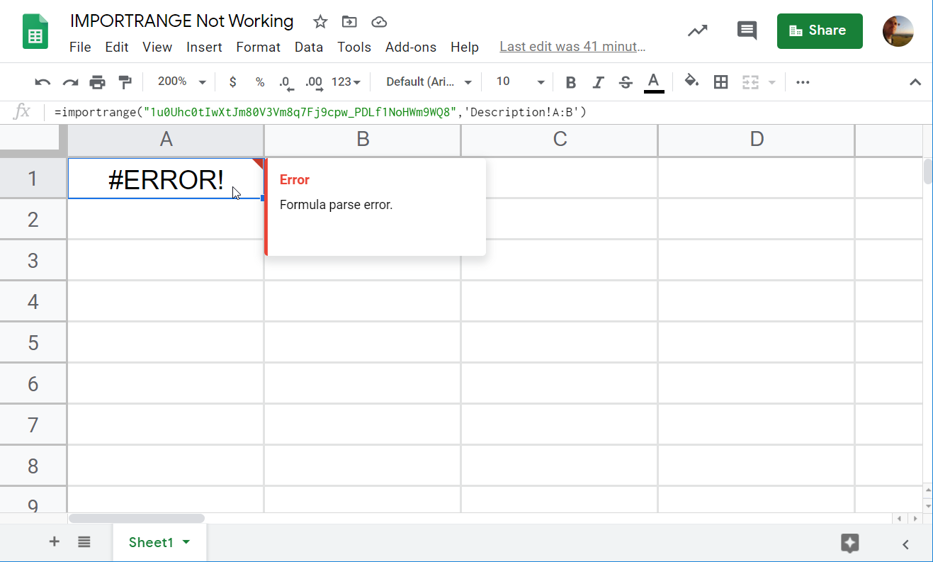
It’s kid’s stuff! Formula parse error means that you’ve made a mistake in the IMPORTRANGE formula syntax.

How to fix

Verify the formula syntax. Make sure also to validate the spreadsheet URL or ID, quotation marks, as well as the range string. These are the most common reasons for the formula parse error.

#2 IMPORTRANGE #REF! – Permission error or You don’t have permissions to access that sheet

This error states that “You don't have permissions to access that sheet.” In most cases, this means that you’re trying to import a dataset from an unshared Google Sheets doc that is not stored on your Google Drive. 

How to fix

Share the source spreadsheet with the owner of the target spreadsheet or make the file shareable with “Anyone with the link.“

#3 IMPORTRANGE #REF! – Allow access or You need to connect these sheets

This is more of a warning than an error. When you import a range from an unshared spreadsheet stored on your Google Docs for the first time, IMPORTRANGE will require you to connect the source and the target sheets.

How to fix

Click the Allow access button to connect the sheets.

#4 IMPORTRANGE #Error! – IMPORTRANGE Result too large

You’ll see this error when you’re importing too many cells. Unfortunately, the exact amount of cells you can import with IMPORTRANGE is undisclosed. In our example, we tried to import 60 columns and 6000 rows (360,000 cells). After we decreased the data range to 4300 rows (258,000 cells), the IMPORTRANGE formula worked. 

How to fix

Split the data range into two or more pieces, either vertically (by rows) or horizontally (by columns). Nest IMPORTRANGE formulas for each piece within the ARRAYFORMULA function as follows:

For horizontally split pieces (use commas between IMPORTRANGE formulas):

=ARRAYFORMULA({IMPORTRANGE("sheet-id","data-range-piece#1"),IMPORTRANGE("sheet-id","data-range-piece#2"),...})

For vertically split pieces (use semicolons between IMPORTRANGE formulas):

=ARRAYFORMULA({IMPORTRANGE("sheet-id","data-range-piece#1);"IMPORTRANGE("sheet-id","data-range-piece#2");...})

For example, here is a failed IMPORTRANGE formula:

=importrange("1bS7FGBbA7nInZJ2VBMaPxqf5B35RXpn-Z3vEcHlTwQo","Data!A:BH")

We split the range of cells "Data!A:BH" by columns into "Data!A:AM" and "Data!AN:BH" and applied the following formula:

=arrayformula({importrange("1bS7FGBbA7nInZJ2VBMaPxqf5B35RXpn-Z3vEcHlTwQo", "Data!A:AM"),importrange("1bS7FGBbA7nInZJ2VBMaPxqf5B35RXpn-Z3vEcHlTwQo", "Data!AN:BH")})

#5 IMPORTRANGE #REF! cannot find range or sheet for imported range

If you see the #REF! Error with a note “Cannot find range or sheet for imported range”, it’s most likely that either the sheet name is misspelled or you entered the wrong range. 

If the formula worked before and then you saw this error, then the sheet was probably renamed or deleted, or the spreadsheet was removed. 

How to fix

First of all, double-check the name of the sheet (both in the IMPORTRANGE formula and your source spreadsheet) and the range you entered. In the vast majority of cases, this is the reason for this internal IMPORTRANGE error.

#6 IMPORTRANGE #REF! – Frozen formulas 

This glitch is well-known among Google Sheets users. Yesterday, your IMPORTRANGE formulas worked well. Today, they return #REF! and seem to be broken for no reason. 

It happens randomly and sometimes fixes itself. For many years, Google has failed to find a stable solution to get rid of this ongoing issue with IMPORTRANGE. 

How to fix

There are many approaches to fixing this issue:

• Hard refresh of the sheet and/or browser
• Re-adding the IMPORTRANGE formula to the same cell (use the Google Sheets shortcuts Ctrl+X and then Ctrl+V or clear the cell and use Ctrl+Z to restore it)
• Nest IMPORTRANGE with IFERROR

=IFERROR(IMPORTRANGE("sheet-id","range"))

The sheet will reattempt the data import again and again automatically.

• Use the =now() trick:
  • Insert a NOW formula (=now()) in a random cell of the source and target spreadsheets
  • Insert an IMPORTRANGE formula that references the NOW formula of the other spreadsheet
  • Go to File => Spreadsheet settings => Calculation and select Recalculation “On change and every minute“
• Split large chunks of data into pieces using ARRAYFORMULA + IMPORTRANGE, just like with Error! Result too large. 

If you know other solutions/approaches to dealing with IMPORTRANGE #REF!, please share them with us to include in the article. 

If you need more information about this function, check out our IMPORTRANGE Tutorial.

How to fix all IMPORTRANGE errors at once: A peace of mind solution

The best way to solve the IMPORTRANGE Google Sheets not working issue is to avoid it. Let’s say you have 100 source sheets from which you import data to 30 sheets using IMPORTRANGE formulas. From the target sheets, you import data to another 10 sheets again with IMPORTRANGE. If all these formulas are stuck, you will face issues with troubleshooting and fixing them! 

IMPORTRANGE is a function, and it takes some time to process calculations, which slows down the general performance of a spreadsheet. Instead, you can use the IMPORTRANGE alternative – Google Sheets integration. It is free of the mentioned IMPORTRANGE performance issues since no calculations are performed in the spreadsheet. It pulls the static data and saves it in your spreadsheet, just in case anything goes wrong.

To set up the Google Sheets integration, you need Coupler.io, a solution to import data from third-party data sources such as spreadsheets, CSV files, and numerous apps. It is available as a web app and a Google Sheets add-on. For the latter, you’ll need to install Coupler.io the add-on from the Google Workspace Marketplace.

Import data using Google Sheets integration

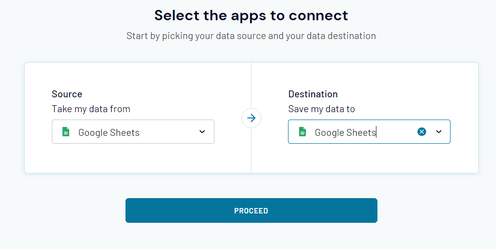
Sign up to Coupler.io, click Add new importer, then select Google Sheets as both source and destination apps.

Check out other available destinations, Microsoft Excel and BigQuery, as well as sources the list of which counts more than 60 and keeps growing. 

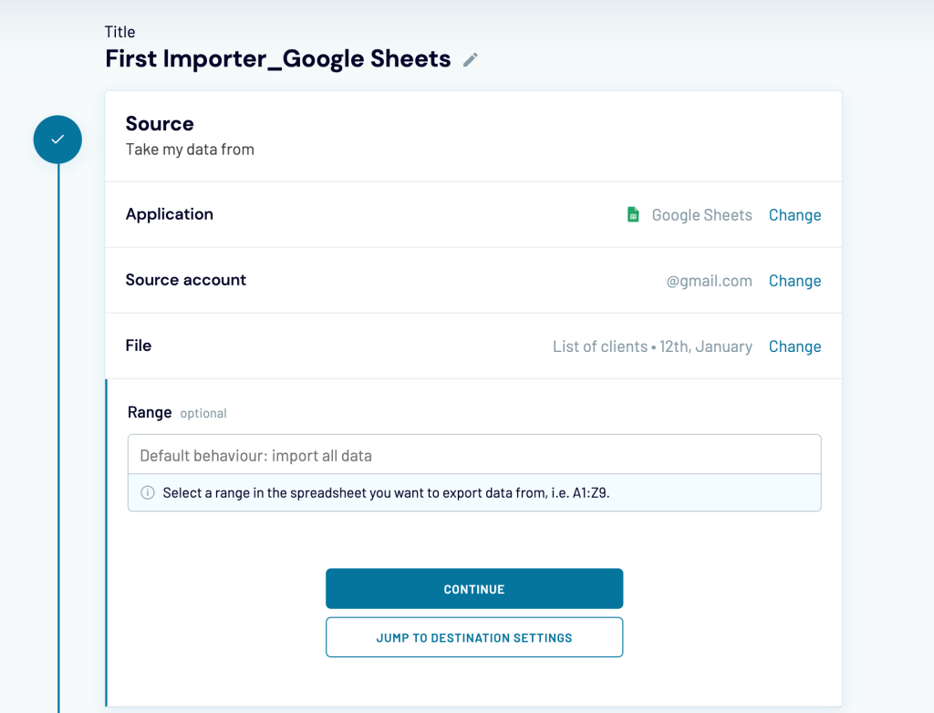
Source

• Connect to your Google account and select a file on your Google Drive and a sheet to transfer source data from. You can select multiple sheets that will be merged into one master view.

Optionally, you can choose a range of data in the spreadsheet you want to export data from, i.e. A1:Z9.

Destination

• Connect to your Google account and select a file on your Google Drive and a destination sheet to transfer data to. You can select an existing sheet, or enter a name to create a new sheet. 

Optionally, you can choose the import mode for your data: you can replace your previous information or append new rows under the last imported entries. Read more about optional destination setup features.

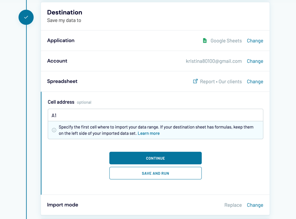
You can run the import right away if you click Save and Run. If you want to automate data import on a schedule, toggle on the Automatic data refresh and customize the schedule.

Schedule

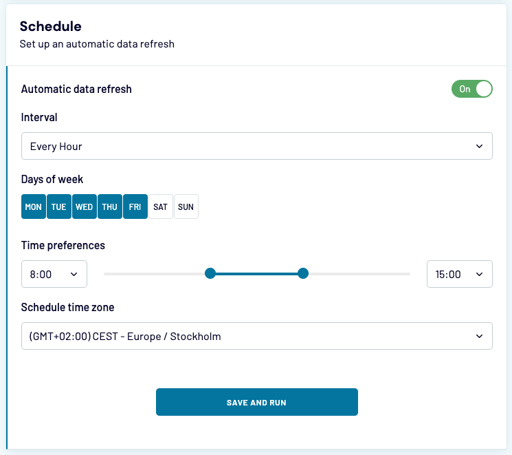
• Select Interval (from 15 minutes to every month)
• Select Days of the week
• Select Time preferences
• Schedule Time zone

In the end, click Save & Run and welcome your data to the spreadsheet. 

How frequently is IMPORTRANGE Google Sheets not working?

Although IMPORTRANGE is an awesome Google Sheets function, its reliability is arguable. Google does not publicly disclose information on the failures of individual functions. However, like any software, you can experience occasional errors when using Google Sheets. So, we can’t be sure how frequently IMPORTRANGE Google Sheets is not working. 

Meanwhile, if you ask StackOverflow about any errors or failures associated with IMPORTRANGE, you’ll get many results starting from 2015. As a rule, such bugs or glitches are solved within a day or two. It’s not a long term but it’s much better not to experience this at all. This is why we recommend you consider the ETL solution by Coupler.io as an alternative to IMPORTRANGE for your project. Check it out and good luck with your data!

Back to Blog

In this article, we will explore why the google sheets IMPORTRANGE not updating.

The IMPORTRANGE is a valuable formula in google sheets when you are working with multiple sheets and you need to reference data from one to another. Many google sheets users report that once they have set the formula working, it does not work the next time.

The IMPORTRANGE formula does update automatically when the source data sheet is open on your computer. It takes a few minutes, but it does update automatically.

Once you have checked these basic things are in place and still, the IMPORTRANGE formula is not updating, then you can try the below trick to update the IMPORTRANGE formula.

Update IMPORTRANGE instantly

If the basic checks are in place and you have waited a few minutes after opening the google sheets, then you can try to recalculate the IMPORTRANGE formula manually.

Here are the steps to solve

1. Open google sheets on your computer

5. Click on save settings

Do these steps for both the source data spreadsheet and destination data spreadsheet. 

Now wait for a few minutes and you should see the IMPORTRANGE formula is now updated.

The trick here is to force a recalculation of the formula. The default settings for the IMPORTRANGE formula to recalculate is 30 minutes when you pull the data from outside the spreadsheet.  

For ImportHtml, ImportFeed, ImportData, ImportXml formulas it is 1 hour. For GoogleFinance it may be delayed up to 20 minutes.

Note, you’re limited to a maximum of 50 of ImportData functions in a single spreadsheet (link).

Wrapping up

In this article, we learned how to solve google sheets IMPORTRANGE not updating issues. While there is a default setting for IMPORTRANGE formula update in google sheets, you can recalculate the formula using the options in settings.

I hope this helped you solve the issue with google sheets importrange not updating. Do write in comments if you still see the issue.

Further Reading

New to google sheets ? Start here